Why the Borwein Integral Pattern Breaks

A sequence of integrals appears to equal π each time, then suddenly falls just short. The discrepancy is so small that a researcher reportedly suspected a computer-algebra bug. The phenomenon is real, and the explanation connects moving averages with Fourier transforms and convolution.

Start with sinc(x) = sin(x)/x, defined continuously as 1 at zero. Its integral over the real line is π, with areas below the axis counted negatively. This is already a surprising result if you approach it using elementary integration techniques.

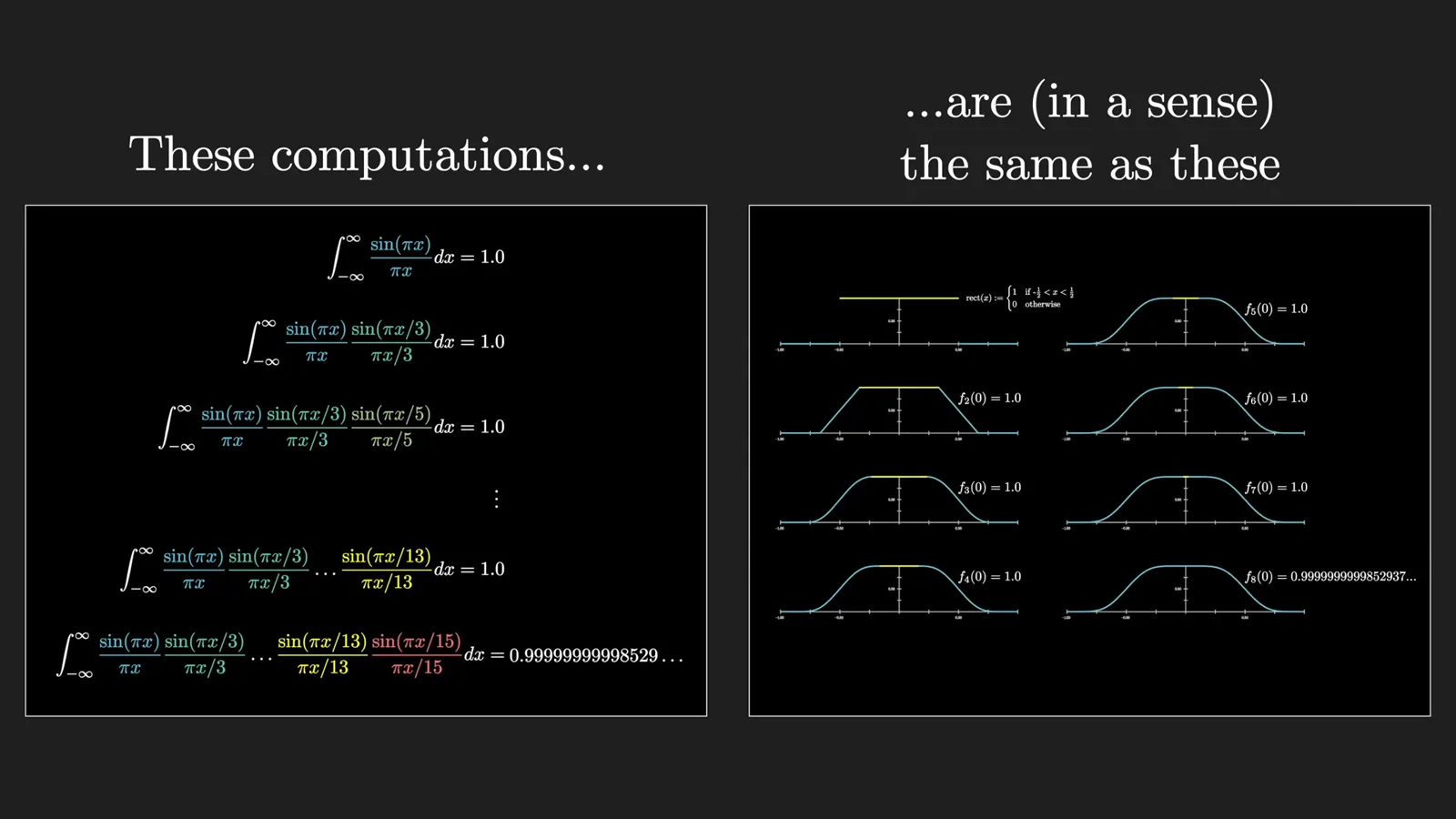
Now multiply by sinc(x/3), then by sinc(x/5), and continue with successive odd denominators. Each factor changes the graph, yet the integral stays exactly π through the factor with denominator 13. Adding the factor with denominator 15 makes it slightly smaller.

The tiny difference is not floating-point error; the exact answer is a rational multiple of π just below π. The Borweins also considered a version with a factor 2 cos(x), whose corresponding pattern persists much longer before breaking at 113.

The video description corrects the display at 4:12: its top line should not be included because that integral diverges. The later valid expressions are the focus of the longer-lasting pattern.

To see a related phenomenon, define rect(x) to be 1 between −1/2 and 1/2 and 0 outside. Create a second function by taking a moving average of the first with a window of width 1/3. Where the whole window sits inside the original plateau, the average remains 1.

The new plateau is narrower by the window’s width, so its length is 1 − 1/3. Its value at zero is still 1. Repeat the averaging with a window of width 1/5; the plateau shrinks again, to length 1 − 1/3 − 1/5.

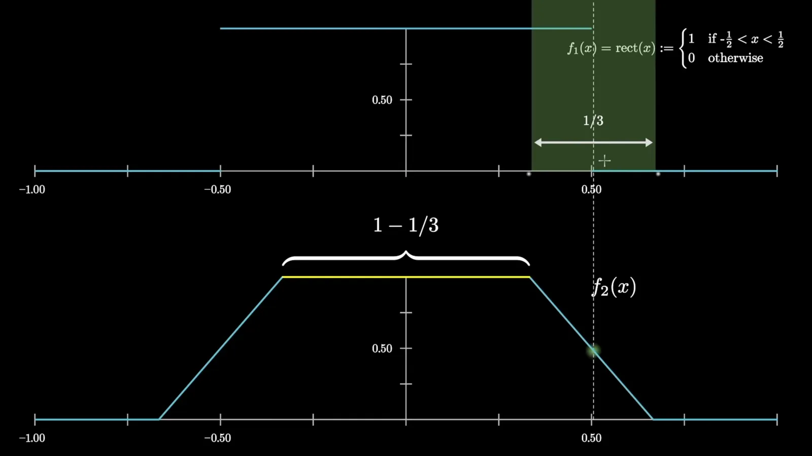
Continue with widths 1/7, 1/9 and so on. The plateau narrows, but near its edge the curve is still very close to 1 because it is built from repeated averages of nearby values.

At the 1/15 step, the previous plateau is narrower than the averaging window. Even at zero the window includes values slightly below 1, so the average drops below 1. This happens because 1/3 + 1/5 + … + 1/15 first exceeds 1.

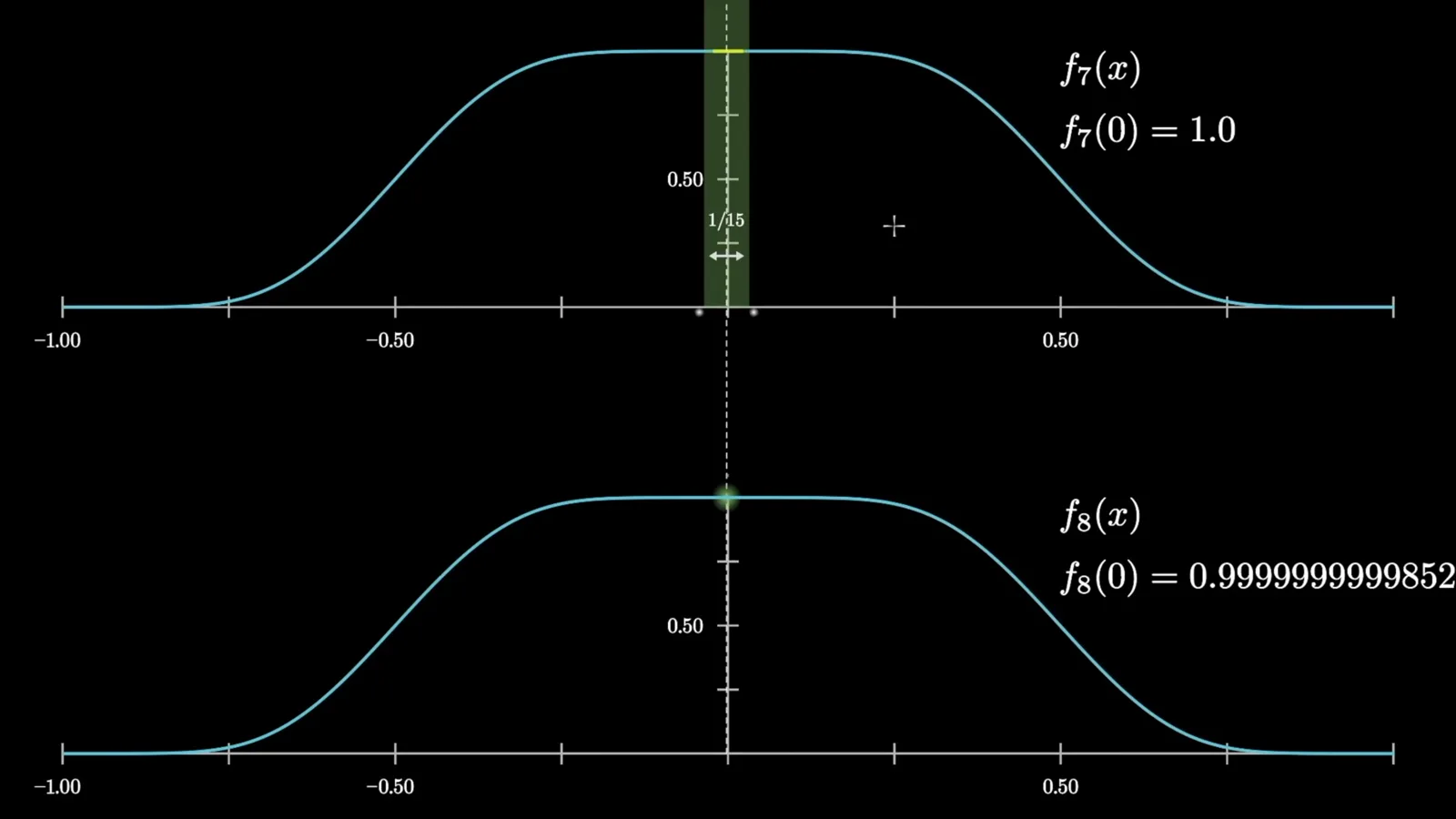
The resemblance is exact: the moving-average value at zero is the factor multiplying π in the corresponding integral. For the 2 cos(x) variant, the analogy starts with a plateau of width 2; the reciprocal sum first exceeds 2 at 1/113.

Odd reciprocals are not essential. The presenter explains the more general principle: for positive scaling values, the plateau remains intact while the total window width is below 1, then the central value falls once it exceeds 1.

Why are the integrals and moving averages the same calculation? The explanation uses Fourier transforms and convolutions. This video gives a high-level overview and leaves a fuller explanation of convolution for a subsequent video.

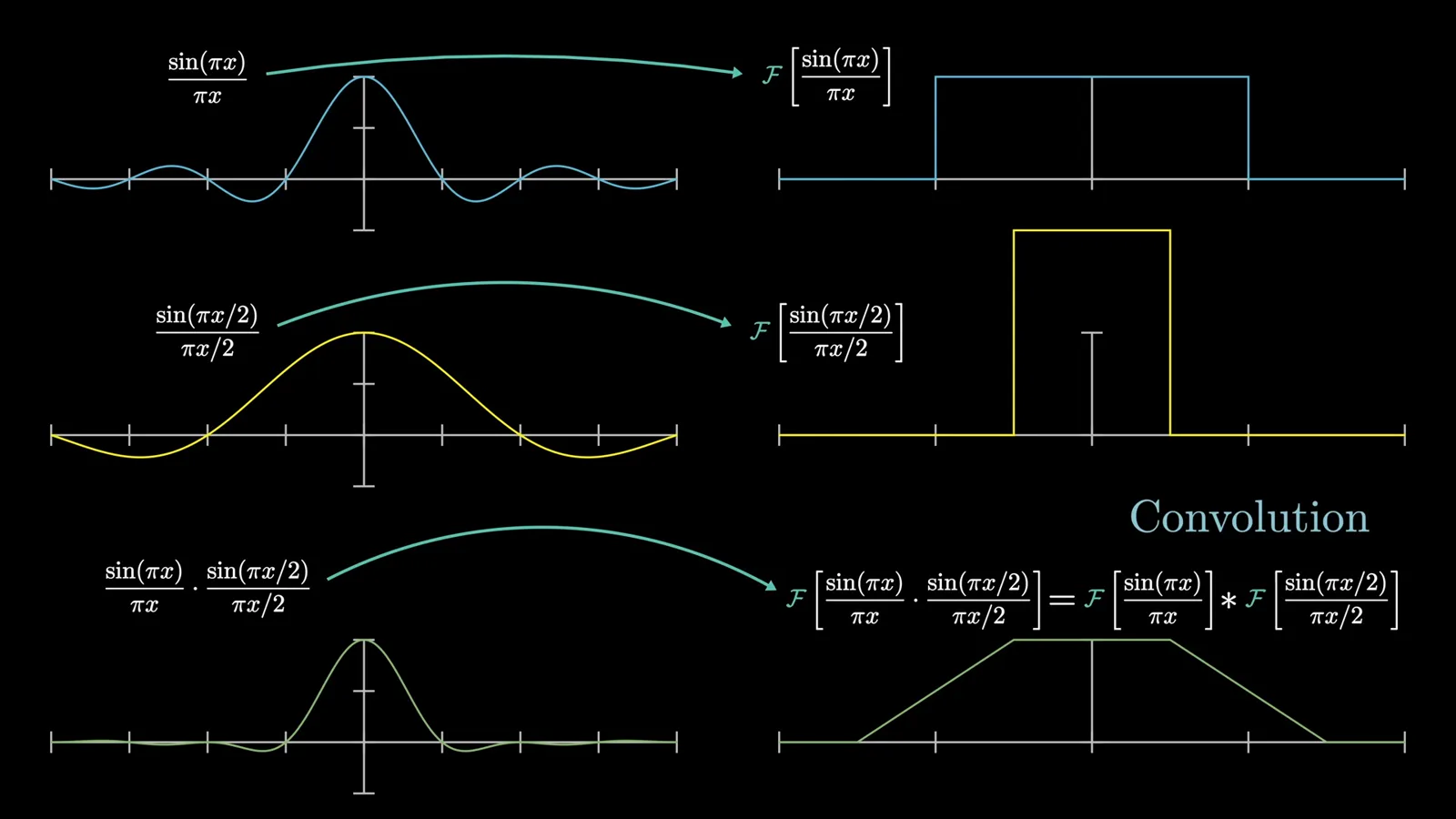
First replace x by πx. This rescales the sinc integral from π to 1. Under the Fourier-transform convention used here, the normalized sinc function corresponds to the rectangular function; a stretched sinc corresponds to a rescaled rectangle.

A Fourier transform can be understood as a change of perspective that expresses a function in terms of its frequency components. Statements that are difficult in the original representation can become simpler in the transformed one.

One useful fact is that the integral of a function over the whole line equals its Fourier transform evaluated at zero, under the convention used in the video. Thus the normalized sinc integral corresponds to evaluating rect at zero, which gives 1.

The convolution theorem supplies the other link: transforming a product corresponds to convolving the transforms. In this example, convolving with the relevant rectangular functions is the moving-average operation. Evaluating at zero therefore connects the product integrals to the shrinking plateaus.

The presenter acknowledges that these transform facts need more justification and promises to explore them in the next video. He adds that the convolution theorem has applications beyond this puzzle, including algorithms for multiplying large numbers efficiently.