How LLM systems fit large models into hardware and serve them faster

Afshine Amidi introduces the problem of training and serving large language models at scale. Decoder-based transformers contain attention and feedforward operations dominated by matrix multiplications, a workload well suited to parallel GPU hardware.

A GPU has many cores and specialized operations for matrix multiplication. Individual entries of a matrix product can be computed in parallel, allowing the hardware to use that parallelism.

He distinguishes a count of floating-point operations from floating-point operations per second, a measure of hardware throughput. GPU specifications also report memory capacity and the bandwidth for transferring data.

For an illustration, a 100-billion-parameter model stored at two bytes per parameter needs about 200 GB just for weights. That exceeds the cited H200 memory capacity; training also requires activations, gradients and optimizer state.

The lecture asks two practical questions: how to fit a model into available hardware and how to make it run quickly. FlashAttention first addresses computation within a GPU; later sections distribute work and optimize inference.

In causal self-attention, each token attends to itself and preceding tokens. The query–key product can produce an N-by-N score matrix for a sequence of length N, making the intermediate costly to store as context grows.

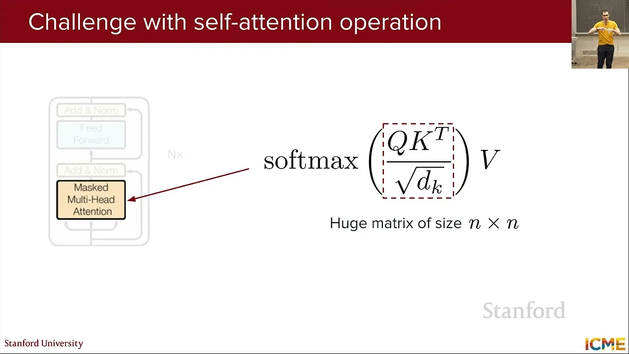
The GPU memory hierarchy matters. High-bandwidth memory, or HBM, is relatively large but slower to access than the much smaller on-chip SRAM used near compute units.

A naive implementation writes and rereads large intermediates from HBM while calculating scores, applying softmax and multiplying by values. The goal is to reduce those transfers rather than assume memory access is free.

Softmax normalizes each score using a denominator containing all entries in the row. At first this seems to require materializing the whole row before computing the result.

Amidi rewrites a single query’s attention output as a weighted numerator divided by a denominator: the sum of exponentiated scores times their values, divided by the sum of exponentiated scores.

Both sums can be accumulated incrementally as new score–value pairs are processed. A three-element example demonstrates updating the numerator and denominator rather than first storing the entire score row.

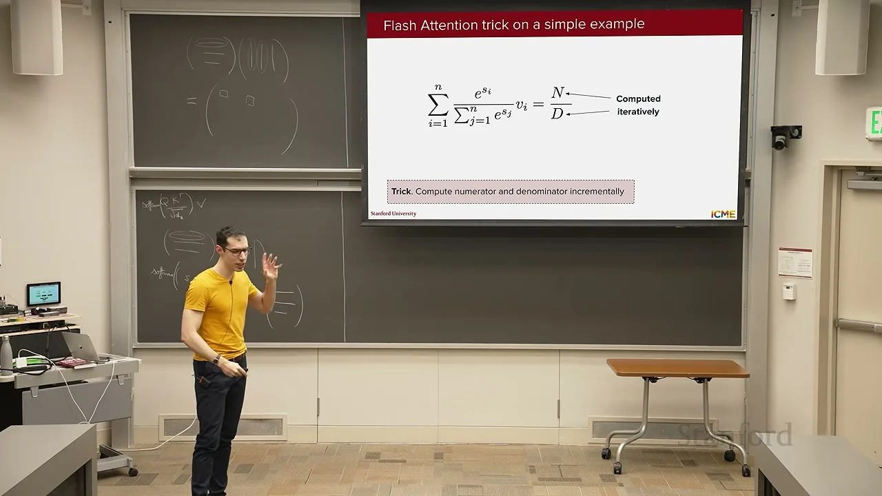
Direct exponentiation can overflow or become numerically unstable. Multiplying numerator and denominator by the same scaling factor leaves their ratio unchanged, so the calculation can be expressed relative to the largest score seen so far.

At the first element, the running maximum is that score. Its exponent can be evaluated after subtracting the maximum, avoiding a need to form a potentially huge exponential before scaling.

When a later score changes the running maximum, the previously accumulated numerator and denominator must be rescaled to the new reference. New terms and old terms must use a consistent scale before the ratio is taken.

The rescaling factor is the exponential of the old maximum minus the new maximum. Amidi shows that this follows from replacing one normalization constant with another; tiny contributions may underflow, but avoiding large overflowing values is the main concern in the explanation.

With this online update, small blocks of queries, keys and values can be loaded into fast SRAM, used to update the running quantities and then replaced. The full N-by-N attention matrix need not be written to HBM.

The resulting attention calculation is mathematically exact in the formulation presented: the algorithm changes the order and placement of operations, not the intended attention formula. As with numerical computations generally, finite-precision arithmetic still applies.

During training, the backward pass needs quantities related to the forward pass. Instead of saving a huge intermediate in HBM, FlashAttention can recompute it from smaller stored information during backpropagation.

Recomputation performs more arithmetic, but can still reduce elapsed time because reading and writing large intermediates is expensive. The example illustrates why minimizing operations and minimizing runtime are not always the same objective.

Amidi notes that later FlashAttention versions introduce further optimizations for different GPU architectures. The core lessons are fused, incremental computation, stable normalization and the tradeoff between recomputation and memory traffic.

Even with efficient attention, a model and its training state may not fit on one GPU. Besides parameters, memory must hold activations for the forward pass, gradients and optimizer state; activations also grow with batch and sequence length.

Data parallelism divides a batch across devices. Each device processes its portion, and gradient updates must be synchronized; a simple version replicates the model and training state on every device.

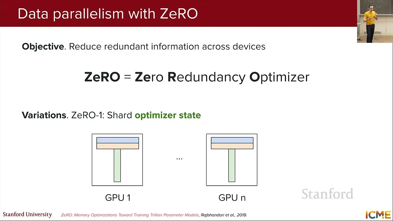
The Zero Redundancy Optimizer, or ZeRO, partitions redundant optimizer state, gradients and potentially parameters across devices. Each GPU stores less, but devices must communicate the pieces needed for computation.

Amidi distinguishes this from model parallelism: in his data-parallel example, a device computes the model for its own sub-batch while retrieving sharded state as needed. Communication has a cost, but can make a model trainable when a full copy will not fit.

Tensor parallelism divides model computations such as matrix operations across devices. Attention heads or pieces of feedforward layers can be distributed, then combined; tensor and data parallelism can be used together.

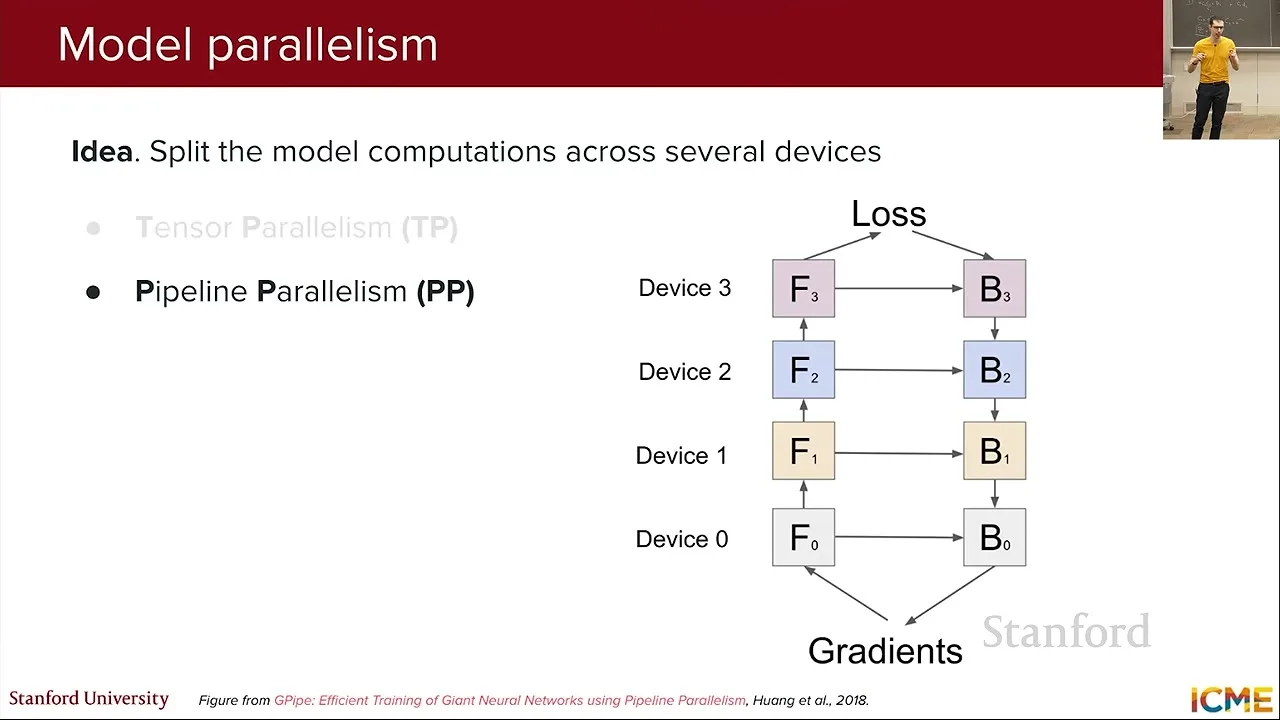
Pipeline parallelism assigns different layers or stages to different devices. Activations move forward through the stages and gradient information moves back during training.

A pipeline can leave GPUs idle while they wait for another stage, a gap often called a bubble. Scheduling strategies try to reduce that idle time, though the lecture does not derive them.

Context parallelism splits work across parts of a long sequence. The example assigns query groups to devices while exchanging key and value blocks so each group can attend to the relevant context.

Expert parallelism applies to mixture-of-experts models. Experts reside on different devices and tokens are routed to the selected expert for the feedforward computation, then returned as needed.

The five dimensions are data, tensor, pipeline, context and expert parallelism. Combining them can help fit and accelerate training, but communication, synchronization and idle hardware limit the benefit of simply maximizing parallelism.

Shervine Amidi turns to inference. A long prompt and short output can behave differently from a short prompt and long output because prompt prefill can process many input tokens in parallel, while autoregressive output is generated sequentially.

He separates queueing time, prefill time and decoding time, and introduces time to first token, time per output token and time to last token. The last metric also depends on output length, including any generated reasoning.

A student asks why prefill is described as fast. The comparison is relative to the number of tokens processed: an individual output step can be short, but many output tokens require repeated sequential steps; cached context can also change prefill work.

For an inference service, speed and cost can be framed as measurable constraints. Amidi introduces compute throughput, memory bandwidth and arithmetic intensity, the amount of computation performed per unit of data moved.

The roofline model relates arithmetic intensity to achievable throughput. At low intensity memory bandwidth can limit performance; beyond the ridge point, available compute can become the limiting factor.

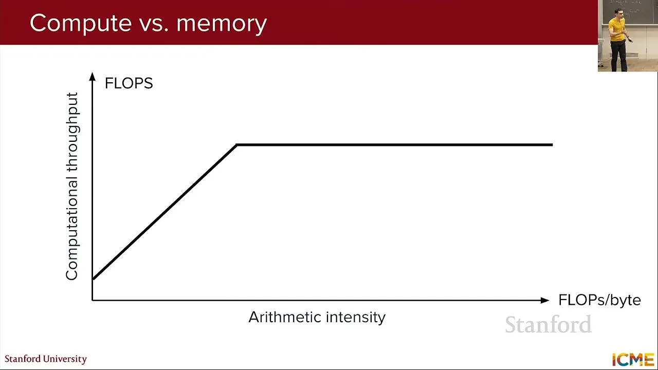
For the illustrated workload, token-by-token decoding often moves substantial model data for relatively little computation and can be memory-bound. Optimized prefill processes more tokens in parallel and can become compute-bound, depending on the workload and hardware.

A KV cache reuses previously computed key and value representations during decoding rather than recomputing them for every new token. Amidi distinguishes that internal decoding cache from provider pricing for reused prompt prefixes across turns.

Naively reserving each request’s maximum possible KV-cache space can leave unused memory stranded when the actual output is shorter. At scale, this fragmentation reduces how many requests can be served.

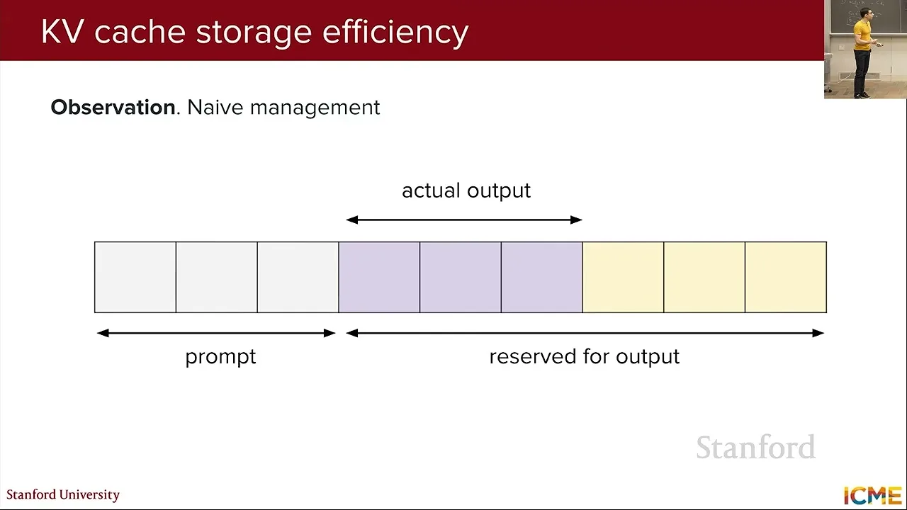
Paged attention divides cache storage into blocks and uses metadata to map logical token positions to physical blocks. Smaller blocks reduce unused reserved space but require more metadata; larger blocks have the reverse tradeoff.

Grouped-query attention reduces the number of distinct key and value heads shared by query heads. With H query heads and G key/value groups, the endpoints recover ordinary multi-head attention at G=H and multi-query attention at G=1.

Reducing key/value groups saves cache memory but changes model capacity, so model designers test the tradeoff. In the lecture’s arithmetic example, two groups for 24 heads reduce the corresponding key/value storage by about 91%.

Multi-head latent attention offers another way to reduce stored key/value information. The lecture describes projecting into a smaller shared latent representation and reconstructing the representations needed for attention, so the compact representation is cached instead.

Speculative decoding targets the sequential generation process. A smaller draft model proposes several tokens, and the target model checks those candidates in parallel, using the difference between parallel verification and serial token generation.

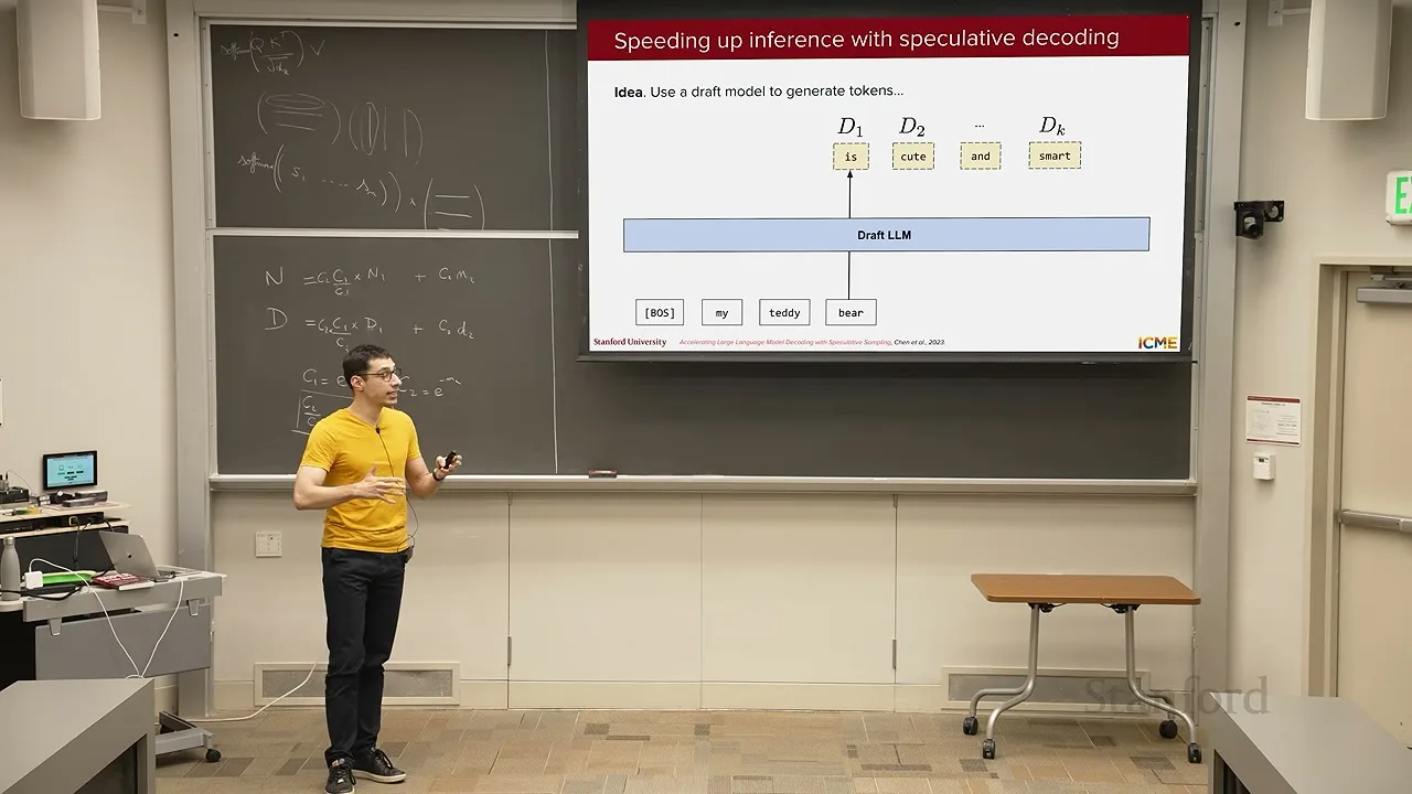
For a proposed token, the described acceptance probability is the minimum of one and the target probability divided by the draft probability. If the token is rejected, the method samples from a normalized residual based on the positive part of target minus draft probabilities.

Amidi derives why this sampling procedure reproduces the target distribution. The accepted contribution for a token is the smaller of the draft and target probabilities; the rejected branch contributes the positive remainder of the target over the draft.

Adding those two contributions yields the target probability for either ordering of the probabilities. This establishes the distributional result for the described procedure, rather than merely trusting that the draft is usually correct.

Verification can also produce a next-token distribution after accepted candidates. Rejections waste draft work after the rejection point, so a draft distribution closer to the target can improve efficiency.

Knowledge distillation is one way to train a smaller draft to match a target’s predictions. The lecture also describes multi-token prediction heads as another way to propose multiple tokens using a model’s own representations.

The instructors close by relating the techniques to their original questions: paging and compact key/value representations help memory fit; parallelism, reduced memory traffic and verifying multiple proposed tokens can improve speed. The best tradeoff depends on workload and hardware.