How particle filter SLAM separates a robot’s path from its map

Marco Pavone contrasts two practical representations of a belief: a parametric approximation such as a Gaussian distribution, and a nonparametric collection of particles. Particles can accommodate multiple modes and nonlinear transition or measurement models.

The class has used particle filters for robot localization and an extended Kalman filter, or EKF, for simultaneous localization and mapping. This lecture applies a particle approach to SLAM, drawing primarily on the Thrun, Burgard and Fox textbook.

The full SLAM problem asks for a probability distribution over the robot’s entire trajectory and the map, given the history of controls and measurements. Pavone contrasts it with the online EKF formulation discussed earlier, which estimates the current state and map.

A naive approach would sample the full joint posterior over the robot trajectory and every feature position. The dimension grows with the map, and the particles needed to represent the distribution can grow prohibitively, an instance of the curse of dimensionality.

The crucial SLAM property is conditional independence: if the robot’s true path were known, the positions of individual map features could be estimated independently under the model. That lets the map problem be broken into lower-dimensional subproblems.

Particle filter SLAM uses particles for possible robot paths and, conditional on each path, an EKF for each feature. It is therefore a hybrid: a nonparametric approximation for the path and Gaussian approximations for landmark positions.

Pavone introduces notation in which the trajectory is the sequence of robot states through time, and the map vector contains the positions of N features. The full posterior factors into the path posterior multiplied by feature posteriors conditioned on that path.

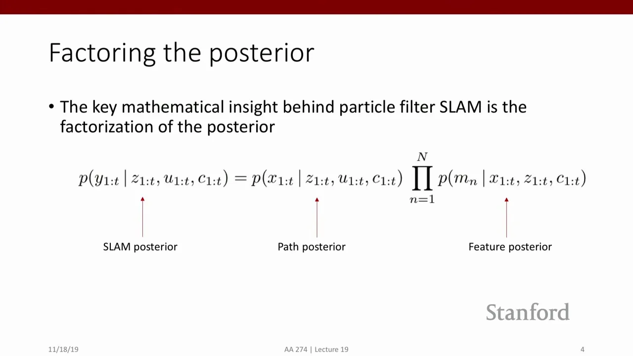
The multiplication of individual feature distributions follows from their conditional independence, not from an assumption that features are unconditionally independent. If the robot’s path is uncertain, estimates of features can still be correlated through that uncertainty.

Each of M particles represents a trajectory hypothesis. Each hypothesis carries N separate feature filters, so the method has M times N small EKFs in addition to the particle representation of the path.

A student asks whether a particle represents its history as well as its present state. Pavone says it represents a full path hypothesis, built incrementally; a later implementation detail is that previous states can be reconstructed with back-pointers.

Although thousands of small filters may sound worse than one filter, Pavone says their low dimensionality makes updates easier. Factoring the posterior exploits an exact conditional-independence property of the SLAM model; the EKF representations themselves remain approximations.

He illustrates the independence with a Bayesian network. A noisy observation depends on the robot’s state and the observed feature. An oracle providing the exact trajectory would remove the shared uncertainty that couples estimates of separate features.

To derive the result, Pavone first separates the joint trajectory-and-map posterior using conditional probability: the path posterior times the map posterior given that path. Other available variables remain in the conditioning where appropriate.

He then removes controls from the feature-estimation conditioning once the path and measurements are known. The next challenge is to show that the posterior over the whole feature vector is itself a product of individual feature posteriors.

As an intermediate step, he compares a feature estimate at times t−1 and t. If the new observation refers to a different feature, it provides no new information about the feature under consideration, so that individual posterior stays the same.

If the observation does refer to the feature, its posterior changes. Bayes’ rule combines the measurement likelihood with the previous feature estimate, normalized by the probability of the observation.

The simplification relies on a Markov model: the current measurement depends on the current state and observed feature, rather than the full state history once those variables are known. Earlier measurements still contribute through the previous posterior.

A student asks why the current state can be omitted from part of the prior term. Pavone explains that, in that term, the new measurement connecting the state to the feature has not yet been included; the relevant information about the feature is carried by earlier measurements.

Pavone turns to mathematical induction to show the factorization holds over time. As a separate example, he proves the familiar sum of the first n integers by checking a base case and showing that the result for n−1 implies the result for n.

For the SLAM proof, he assumes the feature posterior factors through time t−1. Bayes’ rule and the Markov assumptions express the time-t posterior in terms of the new measurement and the earlier feature estimates.

Only one feature in the example corresponds to the latest observation. The remaining feature posteriors are unchanged; substituting the updated expression for the observed feature reconstructs a product over all N features.

Pavone identifies and corrects notation errors on the slides while completing the induction. With a base case and the update step, the factorization holds over time under the model’s assumptions.

With the factorization established, the path posterior is approximated by particles and each landmark posterior by an EKF conditioned on a path. For M path particles and N features, there are M times N landmark filters.

Each particle is accompanied by the mean and covariance of a Gaussian estimate for every feature. Different path hypotheses can therefore carry different maps, rather than forcing all hypotheses to share a single estimate.

A student asks about knowing the number of features. Pavone says the initial presentation assumes known correspondences: the algorithm knows which feature generated each measurement. He returns to unknown correspondences later.

The central update takes the previous set of particles, a new control and a new observation. Pavone divides it into three steps: predict each path, update feature estimates, and correct the path distribution using the measurement.

The first step extends the robot’s path using the motion model and the new control. This is the prediction stage of a Bayes filter; the new measurement has not yet influenced the path samples.

Pavone clarifies the implementation: a current particle need not literally store the entire trajectory as a long vector. A back-pointer to earlier states can reconstruct its history as the filter proceeds.

To propagate a particle, sample a new state from the state-transition distribution conditional on the prior state and current control. The model can produce different possible next positions even from the same starting state.

Next, update the feature filters associated with each path hypothesis. If the latest observation is not associated with a particular feature, that feature’s Gaussian mean and covariance are left unchanged.

For the observed feature, combine the previous Gaussian estimate with the measurement likelihood. The measurement model is linearized, producing the standard EKF update for the feature mean and covariance.

The Kalman gain balances the previous feature estimate against a correction based on the difference between the actual and predicted measurement. The update follows the same algebra already used in EKF localization.

Students ask which covariance belongs to which quantity. Pavone emphasizes that each path particle has its own Gaussian landmark covariances; the robot path distribution is represented by particles, not by a single Gaussian covariance.

A sketch shows multiple possible robot positions and different Gaussian feature estimates attached to each particle. The same landmark can have different means and uncertainties under two path hypotheses.

The path samples so far were propagated using controls, without the latest measurement. Resampling corrects the representation by giving more weight to particles whose predicted observations fit what the robot actually saw.

A path that is highly incompatible with the measurement may be discarded along with the set of landmark filters attached to it. Resampling is performed with replacement, allowing more compatible hypotheses to appear multiple times.

Pavone writes the importance weight as the target posterior divided by the proposal distribution. Bayes’ rule cancels the shared terms, leaving a quantity proportional to the likelihood of the new measurement under the path hypothesis.

The intuition is the same as in Monte Carlo localization: observations favor hypotheses that make the observation plausible. Repeatedly sampling the same hypothesis can cause particle starvation, so sampling strategy matters.

To compute the likelihood efficiently, the measurement model can be linearized and the resulting distribution represented as a Gaussian, as in the earlier EKF and Monte Carlo localization material.

The resulting loop is compact despite its notation: propagate the path for each particle, update the relevant feature filters and compute a weight, then resample the particles using those weights.

A student asks which estimate enters the measurement update. Pavone points to the previous mean for the relevant feature and notes that this portion is the same EKF machinery used earlier in the course.

For unknown correspondences, the filter must decide which landmark produced an observation. Pavone describes maximum-likelihood association: choose the feature that makes the observation most likely for a particular particle.

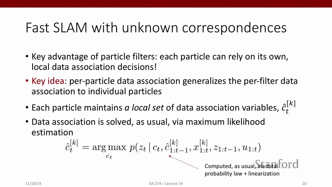
A student asks whether this commits to one association rather than maintaining a belief over possibilities. Pavone explains that the decision is conditioned on the particle: different particles can retain different histories of association decisions.

If an association sends one particle down an implausible path, later measurements may make it unlikely and remove it during resampling. By contrast, a standard single-hypothesis EKF can diverge after a bad association and may need a reset.

Pavone compares the broader approaches. Gaussian filtering represents uncertainty with a Gaussian approximation and linearizes transition and measurement models. It is relatively fast and familiar, but a single mode is a poor representation when several locations are plausible.

He says a Gaussian approach can be adequate when uncertainty is low or the robot is constrained to a narrow setting. A more global localization problem with several plausible modes may call for particles or a different method.

Particle filtering can represent multimodal beliefs and propagate the nonlinear dynamics through samples. Its separate association histories also offer robustness to some data-association errors.

The cost remains significant: even with posterior factorization, many particles may be needed, especially as the state grows. Resampling can also cause particle starvation, motivating more careful sampling methods.

Pavone places SLAM in a longer research history, from EKF approaches through particle filtering and graph-based methods. He describes graph SLAM as using graph optimization, while noting that the class has not covered it.

He recommends a survey that organizes SLAM history from classical filtering, through analysis of algorithm correctness, to robust perception under failures. He also points to OpenSLAM, visual SLAM implementations and benchmark datasets for comparing algorithms.

Closing the localization and mapping module, Pavone returns to the common Bayes-filter pattern: predict, then correct. The main computational tools discussed in the course include linearization, particle representations and posterior factorization.