30초 요약
A language model can help compress text by assigning short codes to likely continuations. Grant Sanderson shows how arithmetic coding repeatedly narrows a region of the number line using those predictions, then sends a binary number inside it so a receiver with the same model can recover the text. The resulting code length connects directly to the cross-entropy used in language-model training. But a fair compression score must also include the decoder and its model; with synchronized updates, adaptation speed can matter too.
- 1A predictable paragraph can contain only a few bits of surpriseKnowing the opening of the U.S. Constitution can make the continuation highly likely; a fixed character code does not exploit that context.
- 2A predictor assigns each message an intervalRepeatedly subdividing the unit interval by the model’s probabilities gives each string a region. A number inside it, together with length and the same model, lets the receiver reconstruct the text.
- 3The same ten bits can encode a longer predictable wordIn the illustrated example, the number for “math” also lies in the region for “mathematics.” The result is unusually lucky and excludes the cost of transmitting length.
- 4Compression depends on the model’s probabilities, not an ideal oracleThe code length approaches −log₂ of the probability assigned by the predictor. A mismatch between that model and real text keeps the result from the true Shannon limit.
- 5The pretraining loss is also a compression costAdding the negative log probabilities of actual next tokens yields a message length; averaging them gives cross-entropy.
- 6A fair score counts the decoder and its modelWithout counting the model, a compressor could hide the data in the decoding program. The Hutter Prize includes that cost.
- 7A compressor can learn while encodingIf the encoder and decoder make identical deterministic updates, a predictor can adapt to new data on both sides without sending each update.
핵심 정리
- Arithmetic coding converts next-token probabilities into a lossless bit stream when encoder and decoder share the same predictor.
- A more predictable continuation generally requires fewer bits; the relevant probabilities are the model’s, which can differ from reality.
- Pretraining cross-entropy corresponds to an average coding cost under this construction.
- Count the decoder and model when comparing total compression, and treat unusually short individual examples as lucky outcomes rather than a new average limit.
- Synchronized deterministic updates let both sides adapt the predictor as the message is processed.
챕터별로 다듬은 전문 읽기
Why predictability should make text smaller
Shannon connects the information in a message to its probability. The challenge is turning that observation into a working code.
An algorithm can compress long stretches of predictable text to less than one bit per character. The Hutter Prize rewards the smallest lossless compression of a gigabyte of Wikipedia, counting the size of the decoder as well as the compressed data. A family of techniques based on the idea we are about to build underlies every winning entry.
Think of compression as two programs: a sender encodes text as bits, and a receiver decodes those bits into an exact copy. To approach the limit, we first need to understand how compressibility depends on the probability of a message.
Claude Shannon showed that the ideal number of bits associated with an event of probability p is −log₂(p). Every time the probability halves, its information increases by one bit. Common messages should need fewer bits than rare ones.
Suppose I give you the beginning of the U.S. Constitution's preamble. If you recognize it, the rest may be very predictable. At a 50% probability, the entire continuation carries one bit of information; even a one-in-a-thousand probability corresponds to only about ten bits.
That seems impossible if we try to assign a fixed bit string to each character. ASCII spends more than 2,500 bits on the passage, and the illustrated Huffman code about 1,500. Even a code for common chunks seems unlikely to fit an entire paragraph into a handful of bits.
The problem is context. A character that is surprising in isolation can be almost certain after a particular prefix. A language model supplies exactly the missing ingredient: for a context it predicts a probability distribution over possible next tokens.
Assume the sender and receiver have the same prediction model. We can plug that model into an encoder and decoder: the better its predictions match the text, the better the compression. The basic idea is to represent a message by a carefully chosen real number between zero and one.
Turn predicted letters into nested intervals
A language model divides a number line according to its predictions. A number in a final interval identifies a message.
For the visual explanation, imagine a model predicting one of 26 lowercase letters at a time. Draw its initial probability distribution as adjacent bars filling the interval from zero to one. Each letter gets a region whose width equals its probability.
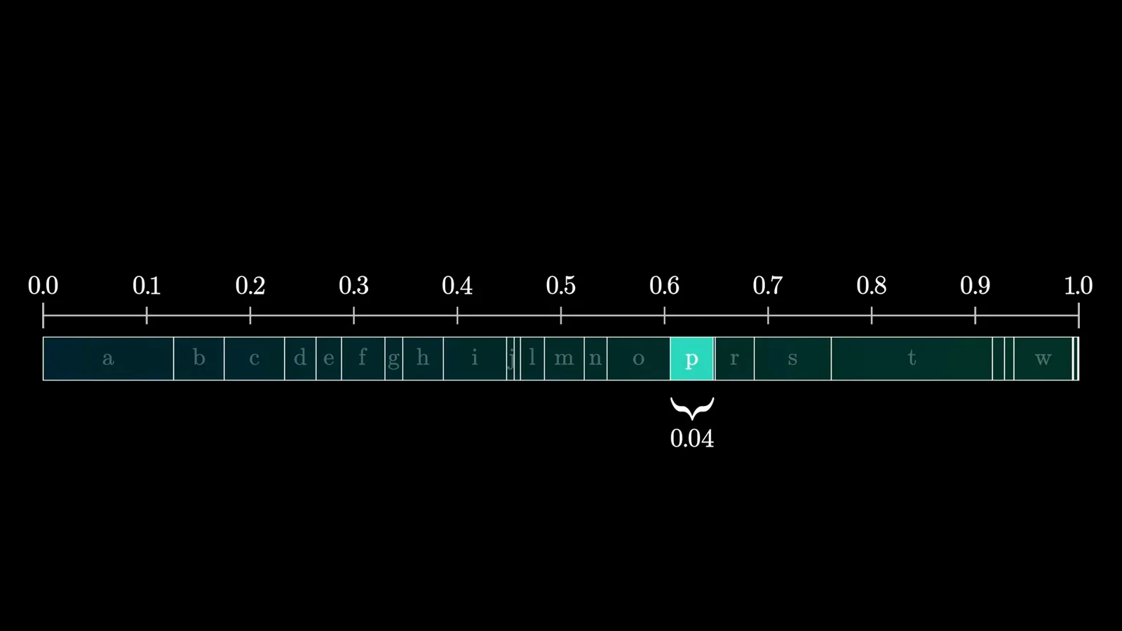
A common initial letter occupies a wide interval; an unlikely one occupies a narrow interval. To encode a longer string, subdivide the chosen first-letter interval according to the model's prediction for the next letter, then repeat inside the selected subinterval.
Take the word 'math.' After choosing the interval for m, ask the model what follows m. The width for ma is the probability of m multiplied by the conditional probability of a after m: the ordinary probability chain rule. Further subdivisions produce intervals for mat and then math.
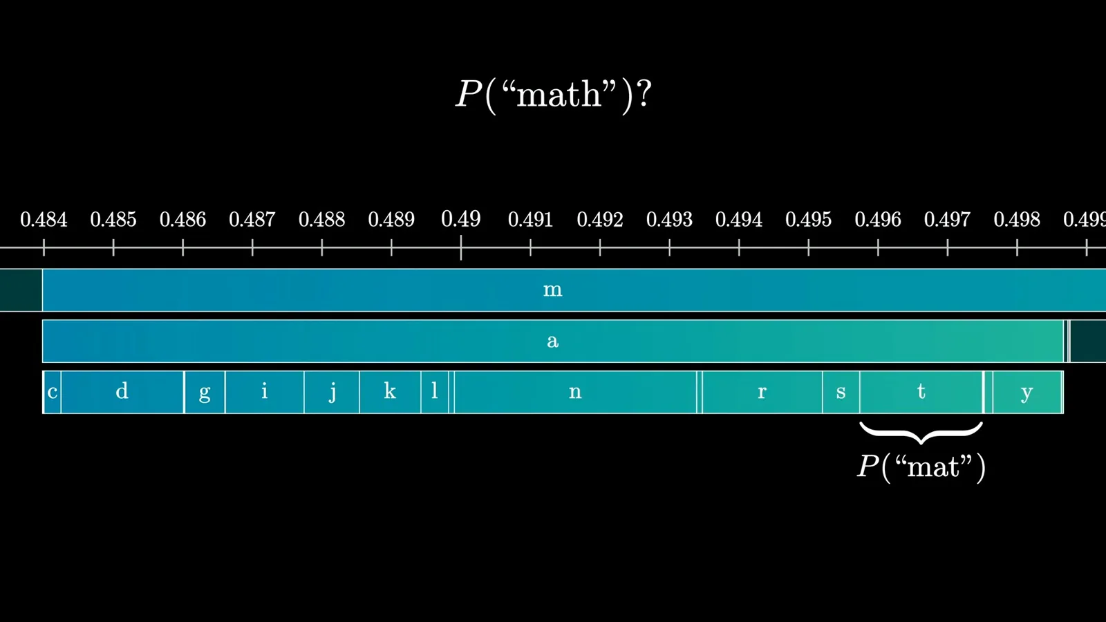
Any number inside the final interval identifies the word, provided the receiver knows that four characters were sent and has the same model. Each additional character selects a smaller nested region; in principle the diagram can continue for arbitrarily long strings.
Decode the number with the same model
The receiver repeats the probability subdivisions to recover each character. Binary precision determines how many bits the number costs.
Decoding reverses the procedure. The receiver starts with the model's distribution for an empty context, locates the number within a first-letter interval, then uses that letter as context for the next prediction. Repeat until the specified length is reached, or use a special end-of-message symbol instead.
If we select numbers uniformly at random from the interval and decode them, the resulting strings tend to look plausible. More likely text receives a larger share of the number line. This is also a way to visualize how a language model generates text.
To transmit an actual number, write it in binary. Each bit halves the possible interval: the first picks a half, the next a quarter, then an eighth. With a finite number of bits we send a point on this binary grid, and it must fall inside the message's target region.
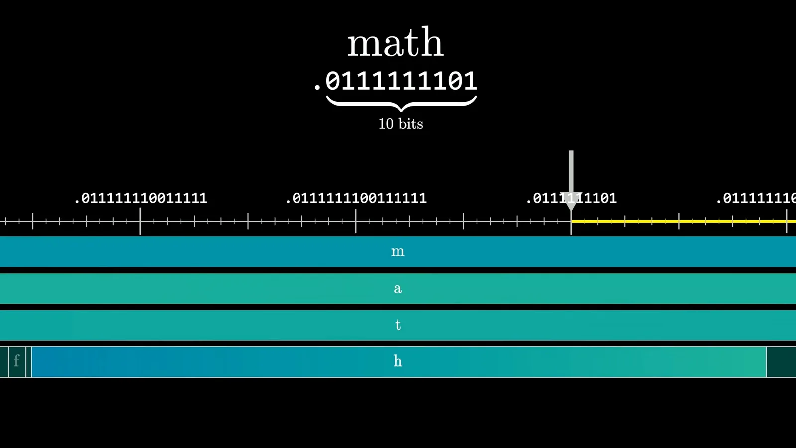
In the illustrated example, a 10-bit number lands inside the interval for 'math'; neither neighboring nine-bit value does. That is 2.5 bits per character, but a longer, predictable continuation can reuse the same number.
Why a lucky ten-bit word does not break Shannon’s limit
The target interval and the binary grid explain the relationship between probability and code length. Message length and model accuracy also matter.
The model strongly expects many letters after 'math,' so the interval hardly narrows as we continue to 'mathematics.' The same ten bits happen to work for all eleven letters, or about 0.91 bits per character, before accounting for the separately transmitted message length.
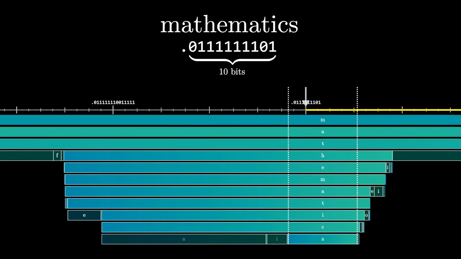
That particular outcome is lucky: the interval for 'mathematics' has width about 2⁻¹⁸, even though a ten-bit grid point happens to fall inside it. In general, binary grid points with at most k bits are spaced 2⁻ᵏ apart.
For a target interval of width p, choosing k at least as large as −log₂(p), rounded up, guarantees a representable point inside without relying on luck. This is why the model-assigned probability translates into roughly that many bits.
The encoded number is not the whole package: the receiver also needs the message length or an end marker. For long messages a fixed-size length header can be small relative to the payload. Some individual strings can use fewer bits than their information value, but Shannon's limit concerns averages.
There is another qualification. The p used here comes from the model, not necessarily from the true distribution of messages. The compression approaches the theoretical limit only when the model's probabilities closely match the actual statistics of the text.
See language-model training as compression
Negative log probabilities add across tokens. Their average is the cross-entropy minimized during pretraining.
Expand the model's probability for a full string into a product of its successive next-token probabilities. Taking the negative logarithm turns that product into a sum: each prediction contributes a cost, large when the actual next token was assigned a low probability and small when it was expected.
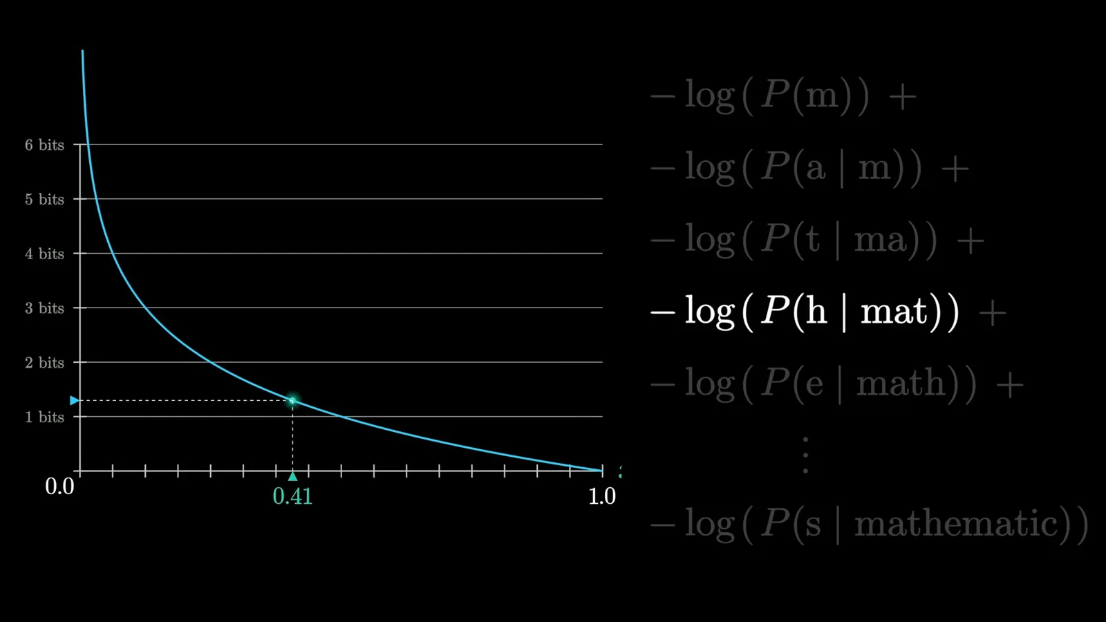
Language-model pretraining minimizes the average of this cost, known as cross-entropy. We can describe the same objective as making a better next-token predictor, or, through this coding scheme, as reducing the number of bits needed to compress the training text.
Compare two predictors and make arithmetic coding practical
A larger predictor compresses illustrative passages more tightly. Practical arithmetic coding rescales intervals to avoid unbounded precision.
A small illustrative NanoGPT model with 3.7 million parameters encodes a sentence about Euclid's Elements in 254 bits, roughly two bits per character. A larger half-billion-parameter Qwen model gives the predictable ending much higher probability and compresses the whole example below one bit per character.
With the U.S. Constitution preamble, the Qwen example uses roughly 35 bits for the opening and only about ten more for the rest. After the opening establishes the context, nearly all of the probability sits on the expected continuation; spelling and capitalization account for some remaining decisions.
There is a fair objection: a model that has effectively memorized a famous passage is carrying information somewhere else. We will return to the cost of the model itself. There is also a practical problem: naively zooming into ever-smaller intervals demands increasing numerical precision.
The conceptual interval method dates at least to Peter Elias's work in 1960. Jorma Rissanen and Richard Pascoe independently developed practical arithmetic coding in 1976. By repeatedly rescaling the working interval, implementations avoid requiring ever-growing precision while retaining the prediction-to-compression idea.
Arithmetic coding provides a nearly ideal way to turn a predictor into a compressor, and improvements in the Hutter Prize have come from better predictors. Yarik Duda's asymmetric numeral systems offer a different approach, using a growing integer and other techniques to obtain fast encoding.
What compression can and cannot say about intelligence
Prediction, compact models and fast adaptation each connect to compression. The proposed definition remains narrower than the ordinary human concept.
The title 'compression is intelligence' should be treated as a proposed mathematical definition, not as a settled statement about everything people mean by intelligence. A useful definition can leave out human nuance while still unifying phenomena that initially seem unrelated.
First, prediction and compression are closely linked. Arithmetic coding turns a predictor into a compressor. In the other direction, we can compare the compressed length of a passage with and without a proposed continuation; a length increase of δ bits suggests a probability of roughly 2⁻ᵟ.
That two-way relationship suggests compression may act as a proxy for prediction. Sanderson connects it to predictive processing in neuroscience, a theory in which the brain forms predictions and passes along differences between prediction and sensory input.
Prediction alone misses another part of what I mean by understanding: explaining many results using a small number of principles. If two models predict equally well, the smaller model suggests a more compact representation rather than an equally large store of remembered details.
Two equally predictive models would compress the same data stream to a similar size, but a fair comparison must include the decoder and its model. Otherwise one could hide a copy of Wikipedia inside the decoder and make the transmitted payload arbitrarily small. The Hutter Prize counts both.
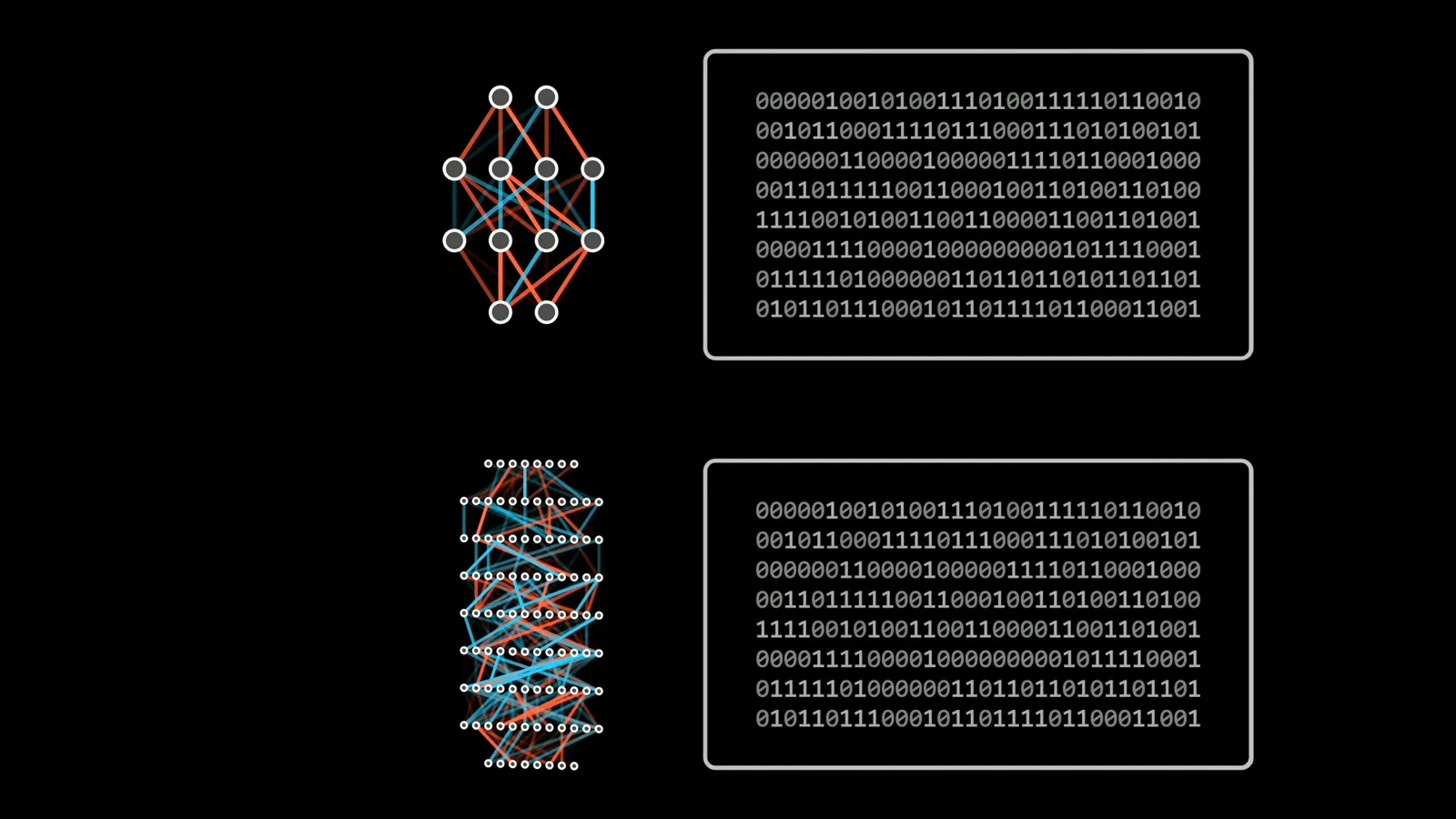
This answers the concern about a large model apparently memorizing the Constitution: its parameters are part of the cost if the recipient needs them to decode. A smaller model with the same predictive performance achieves better total compression.
A third aspect is how quickly a system learns. A fixed model's final compression score says nothing directly about how long training took. But a model trained on Wikipedia could be adapted while compressing a different source, such as Shakespeare.
The encoder can update its model as it sees each token; the decoder performs the identical deterministic updates as it reconstructs them. Their predictions remain synchronized, so a model that adapts quickly to the new material can improve the resulting compression.
The two sides can even begin from the same reproducibly generated random model, avoiding transmission of initial trained parameters. In such an adaptive setup, the score depends not only on static prediction but also on how quickly the model learns from the data it processes.
Across the trilogy, Shannon's estimates of English compressibility required human prediction; modern AI training uses mathematics developed for compression; and strong practical compressors combine prediction, compact models and sometimes rapid adaptation. Compression is not identical to every human meaning of intelligence, but it captures more of the idea than I first expected.
같은 채널의 다른 글
 40:44EN
 3Blue1Brown· 2026년 10월 16일Grant Sanderson: There's never been a better time to go into mathGrant Sanderson, Constantin Kogler · 3Blue1BrownStudents fear AI has solved mathematics. Grant Sanderson argues the opposite: even if machines prove theorems better than we do, the institution of math stays valuable—and this is a rare moment when newcomers can reshape it.
 51:55EN3Blue1Brown· 2026년 9월 18일The last IMO problem AI could not solveGrant Sanderson · 3Blue1BrownGrant Sanderson walks through IMO 2025 Problem 6 — a tiling puzzle that frontier models missed — and the visual patience it takes to prove a construction is optimal.
 0:55EN3Blue1Brown· 2026년 7월 24일The 64 Sugar Cubes Puzzle: Six Equal DistancesA 4×4×4 block has three colors; prove that six same-colored pairs share a distance.
 33:51EN3Blue1Brown· 2026년 7월 16일What Cross-Entropy Connects: Compression, Language Models and KL DivergenceGrant Sanderson · 3Blue1BrownGrant Sanderson builds cross-entropy from code lengths and uses it to explain next-token training and distillation.
 2:25EN3Blue1Brown· 2026년 6월 12일How Shannon Measured the Entropy of EnglishA guessing game helped Claude Shannon estimate how much information English text contains, and why prediction is central to compression.
 1:02EN3Blue1Brown· 2026년 6월 10일A Robot Walk and the Puzzle of Optimal Binary EncodingHow few bits does it take to send directions that occur with unequal frequencies?