Euler’s Formula, Oscillators and the Road to Laplace Transforms

This first chapter of a series prepares for the Laplace transform by building intuition for complex exponentials. The goal is also worthwhile on its own: understand why Euler’s formula and a seemingly strange substitution help solve a differential equation common in physics.

The function e^t equals its own derivative. Rather than viewing that derivative only as a graph’s slope, imagine a point whose position is e^t on a number line. Its velocity always equals its position, and it starts at 1, so it moves right faster and faster.

For e^(2t), the velocity is twice the position, giving faster growth. For e^(−0.5t), velocity points in the opposite direction and is half the position’s magnitude. The point approaches zero more and more slowly: exponential decay.

Now consider e^(it). Its derivative is i times the function. Multiplication by i rotates a complex vector 90 degrees: for a + bi, the product is −b + ai. Thus the velocity is always perpendicular to the position.

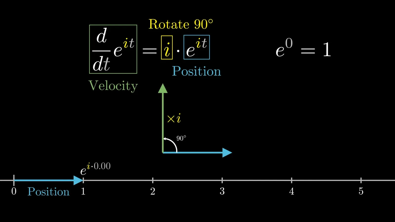
Starting at 1 with velocity equal in magnitude to position, the point moves counterclockwise around the unit circle at one radian per unit time. After π units it reaches −1, giving e^(iπ) = −1. This dynamic picture explains the famous identity.

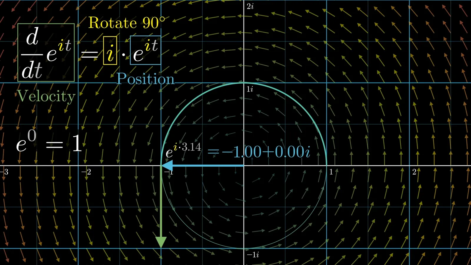
For a complex input, the exponential is not best understood as repeated multiplication. One definition uses its convergent Taylor series. The derivative and initial-value picture makes the resulting circular motion much easier to see than inspecting the infinite sum term by term.

Each point s in the complex plane can represent an entire function e^(st). If s = 2i, the motion rotates twice as fast as e^(it); more generally, the imaginary part gives angular frequency and direction.

When s has both real and imaginary parts, the motion combines growth or decay with rotation. For s = −0.5 + i, the magnitude shrinks while the point spirals. Engineers call the plane of possible exponents the s-plane.

This derivative relationship is itself a differential equation. Reverse the perspective: can a physical differential equation motivate complex exponentials? A mass on a spring is a central example.

Let x(t) be the displacement from equilibrium. Its first derivative is velocity and its second derivative acceleration. A restoring force approximately proportional to displacement points toward equilibrium, while a damping force can be modeled as proportional to velocity.

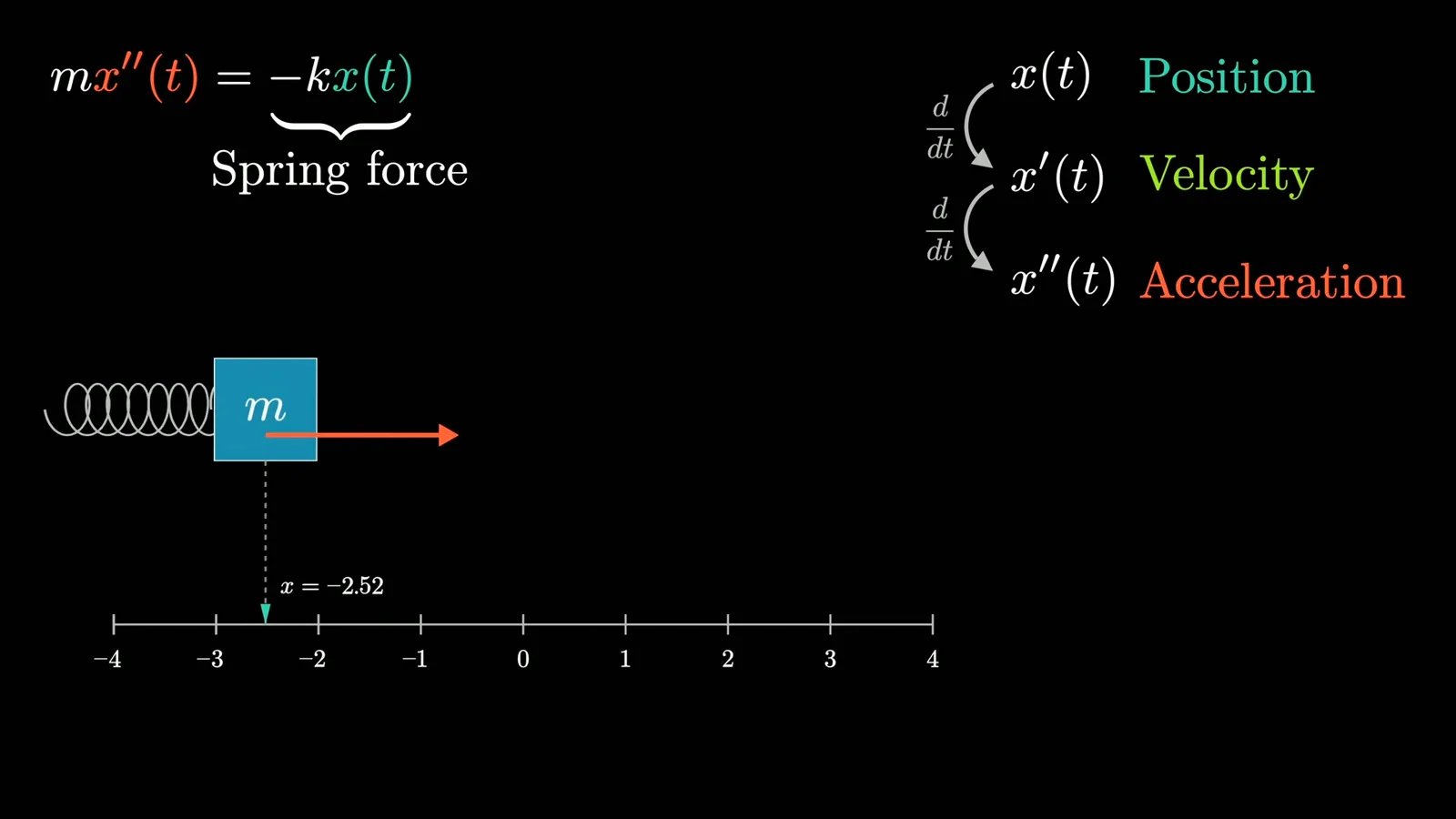
With mass m, damping μ and spring constant k, the homogeneous equation is mx″ + μx′ + kx = 0. Position and velocity at the start select one member from a family of solutions. The simple proportional damping term is an approximation to real resistance.

Try x(t) = e^(st). Differentiating multiplies by s each time, so substitution gives e^(st)(ms² + μs + k) = 0. Since the exponential is never zero, the problem reduces to the characteristic equation ms² + μs + k = 0.

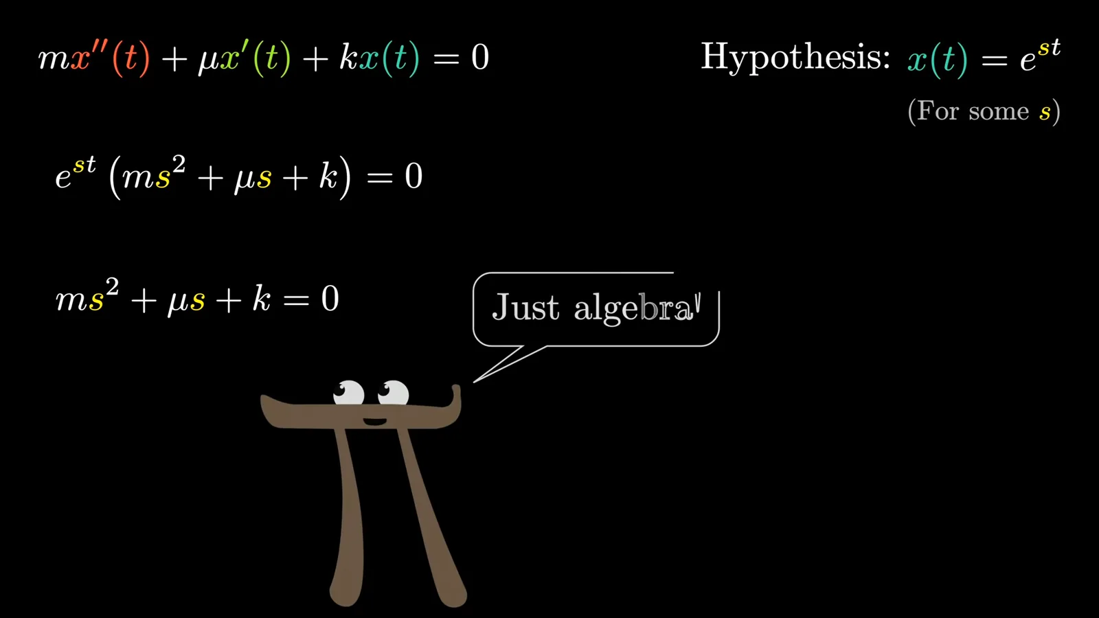
Without damping, μ = 0 and the roots are s = ±i√(k/m). Let ω = √(k/m). The two complex exponential solutions rotate in opposite directions, with a stronger spring corresponding to a higher angular frequency.

The physical position must be real. Taking a real part works, and adding e^(iωt) and e^(−iωt) gives 2cos(ωt). Because the homogeneous equation is linear, scaled sums of solutions are also solutions.

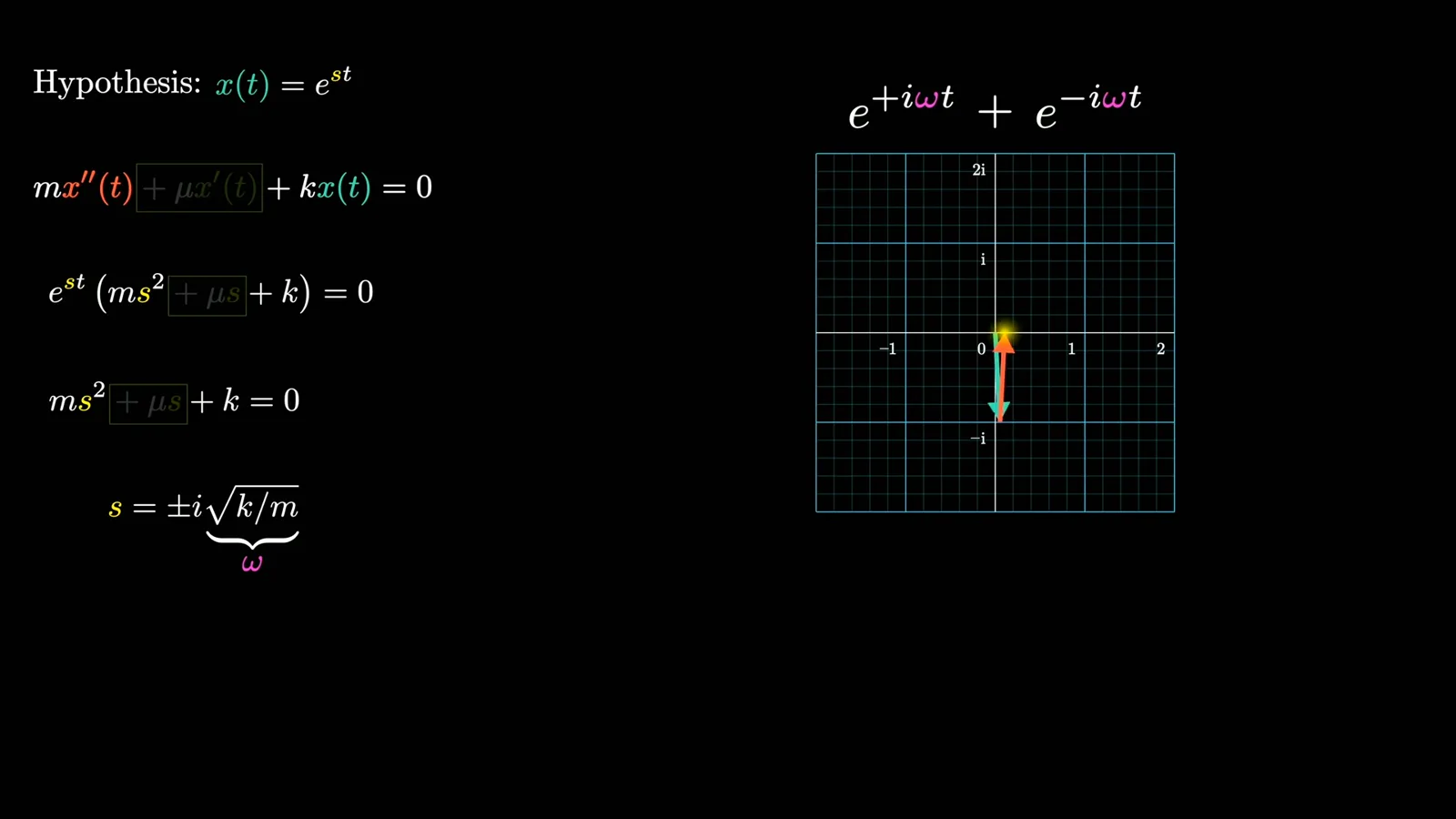
The coefficients can be chosen to fit initial position and velocity. In real terms the same family can be written as A cos(ωt) + B sin(ωt). For example, equal coefficients of one on the two exponentials give initial position 2 and initial velocity 0.

Why use complex exponentials when sine and cosine already solve this simple case? They become especially convenient when the equation changes. Reintroducing damping moves the roots away from the imaginary axis into the left half of the s-plane for positive damping.

In the underdamped case the roots have negative real parts and nonzero imaginary parts. The corresponding motion both decays and oscillates. With sufficiently strong damping the roots are real and negative, producing nonoscillatory decay; the repeated-root boundary needs its own solution form.

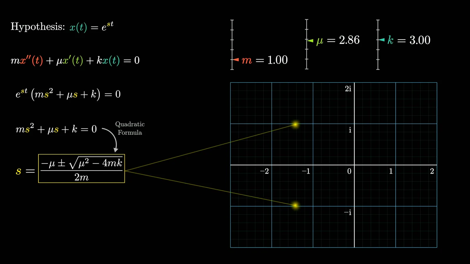
The same substitution works for homogeneous linear equations with constant coefficients and higher derivatives: the differential equation becomes a polynomial in s. Distinct roots yield exponential solutions that can be combined; repeated roots require additional factors such as powers of t.

Many physical problems add an external force. In a model of light passing through material, charges behave like damped oscillators driven by a periodic light wave whose frequency need not match their natural frequency.

The driven equation is still linear, but it is nonhomogeneous. Its general solution combines a particular response to the force with the homogeneous solutions, so the coefficients of the forcing response are constrained. In the illustrated nondegenerate case, the result can be expressed using four exponential terms.

This motivates a systematic question: given a differential equation, how can we identify the exponential pieces and their coefficients? The Laplace transform provides a way to do that and connects the story to Fourier analysis, including continuous combinations of exponentials.

In the next chapters, the transform will translate time functions into a language where differentiation becomes algebraic, with initial-condition terms accounted for. That generalizes the intuition behind the exponential substitution used here.