Stephen Welch: How Diffusion Models Turn Text into Images and Video

AI image and video generators can turn text into remarkably detailed scenes. Stephen Welch introduces diffusion as a connection to Brownian motion run in reverse in a high-dimensional space. The physical analogy leads to practical algorithms, not merely a metaphor.

As an example, Welch shows the open WAN 2.1 video model responding to prompts about an astronaut. Its generation process starts from random noise and repeatedly applies a transformer, gradually shaping the sample into a video. The video description notes that the displayed noise is decoded from a compressed latent representation.

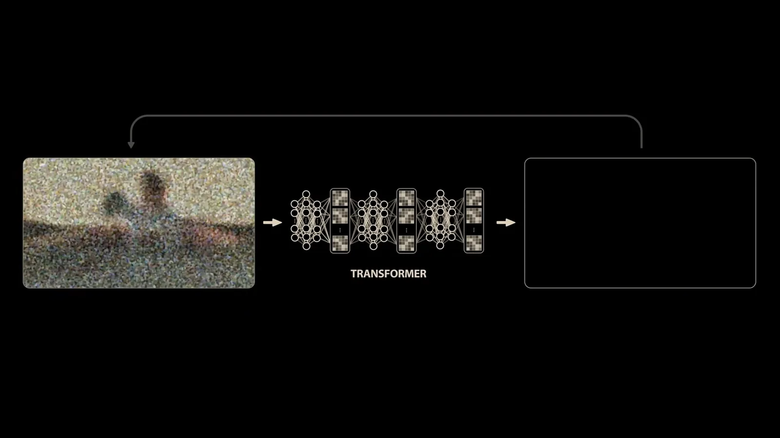
Each model pass produces an update; repeated iterations add visible structure. This raises two questions: how can a model reverse a random process, and how does text steer that process toward a requested scene? Welch approaches them through CLIP, diffusion and guidance.

OpenAI’s CLIP, released in 2021, uses an image encoder and a text encoder trained on image-caption pairs. Each produces a vector in a shared space. The training objective makes matching image and caption representations similar and pushes nonmatching pairs apart.

In a batch, arrange image vectors against caption vectors in a matrix. Matching pairs lie along the diagonal; other entries are nonmatches. The contrastive objective uses both kinds of pair, with cosine similarity measuring how closely the vectors point in the same direction.

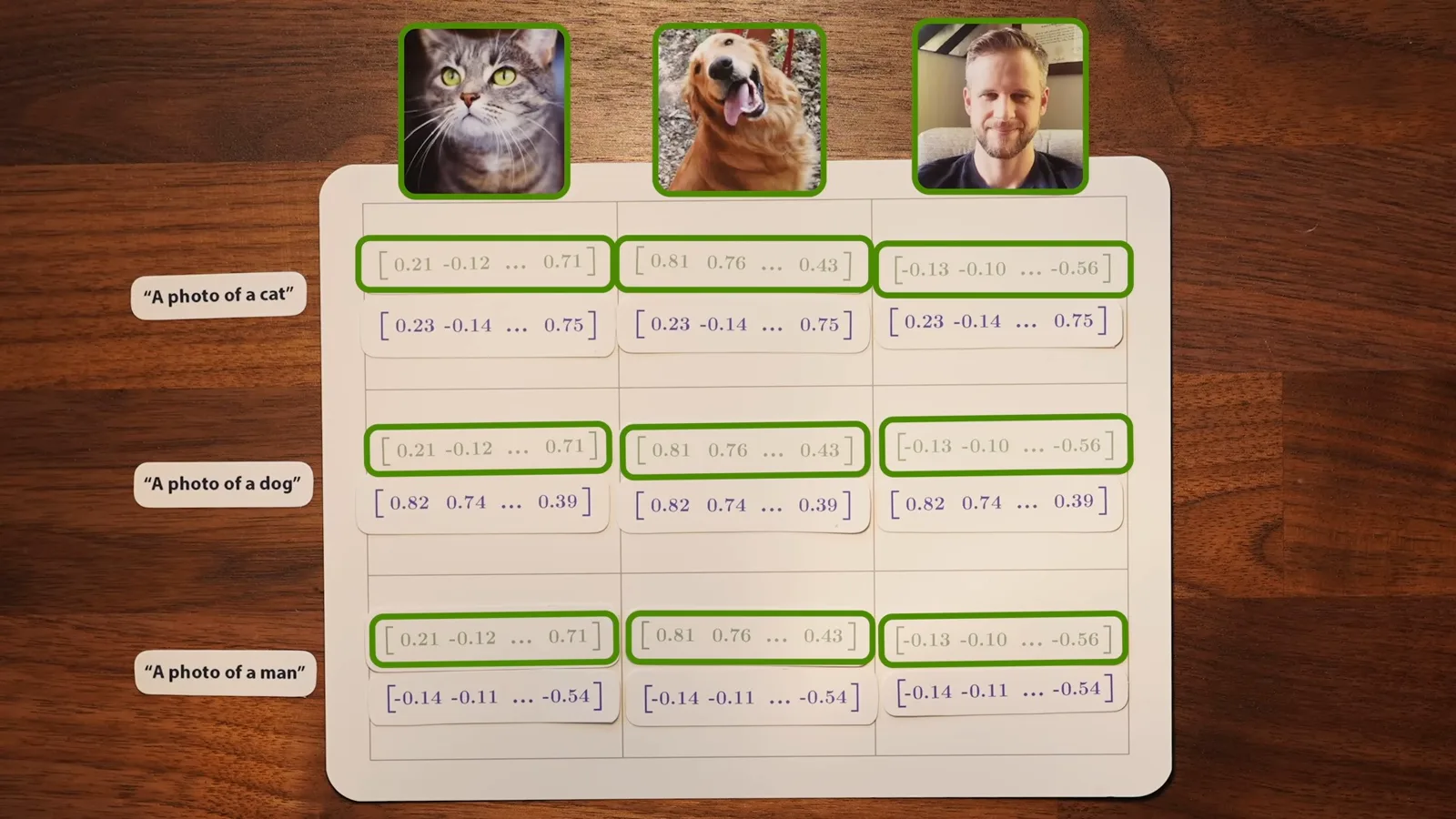
Cosine similarity is the cosine of the angle between vectors; identical directions have similarity one. The learned space lets the model compare descriptions with pictures, even though the geometry is high dimensional and the two-dimensional illustrations are only an aid to intuition.

Welch subtracts the embedding of a photo without a hat from one with a hat. Among several hundred words, “hat” is the strongest match to the difference vector in his experiment, followed by related words. This illustrates that some meaningful image differences correspond to directions in the learned space.

CLIP can classify an image by comparing its embedding with candidate text labels and selecting the most similar one. But these encoders map images and text into the space; by themselves they do not generate an image from an embedding.

Denoising Diffusion Probabilistic Models, or DDPM, provide a way to generate images. Training begins with clean examples and adds scaled random noise. The neural network learns to estimate the total noise added, rather than merely recovering the immediately previous step.

DDPM sampling also adds random noise during generation. In Welch’s Stable Diffusion example, removing that step from the DDPM update produces a small, blurry tree. The video’s technical notes add that a mismatch between the actual and expected noise levels is a likely cause of that particular degradation.

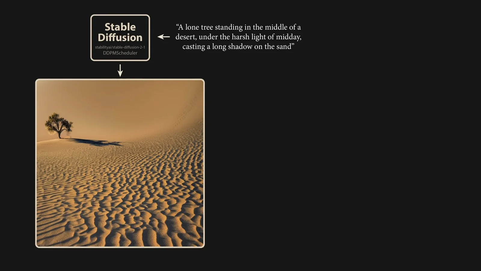
Why predict the total noise rather than only the last small step? Welch uses a different but related view: the model learns a time-varying vector field that directs noisy samples toward the data distribution. That view also connects to broader flow-based approaches.

Imagine an image with only two grayscale pixels. Their intensities become x and y coordinates on a plane. A collection of images becomes a set of points; for the toy example, Welch arranges them along a spiral.

Adding noise changes pixel values in random directions. Repeated additions move a point on a random walk, analogous to Brownian motion. Learning to denoise means learning how to move noisy points back toward the spiral’s distribution, not reconstructing the particular random path exactly.

For a given noisy point, many possible training paths may have passed nearby. Although each final step is random, their average contains a direction toward the data. Predicting total added noise gives a lower-variance training signal for learning this direction.

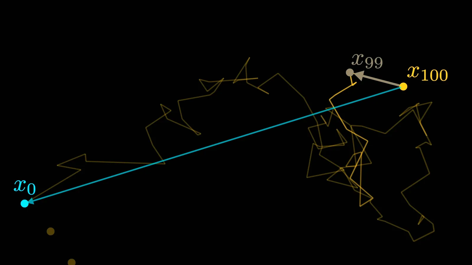
The learned direction also depends on the noise level. Far from the original data the field points broadly toward the spiral’s center; at lower noise it can resolve finer structure. Providing the time or noise level as an input lets one model learn both.

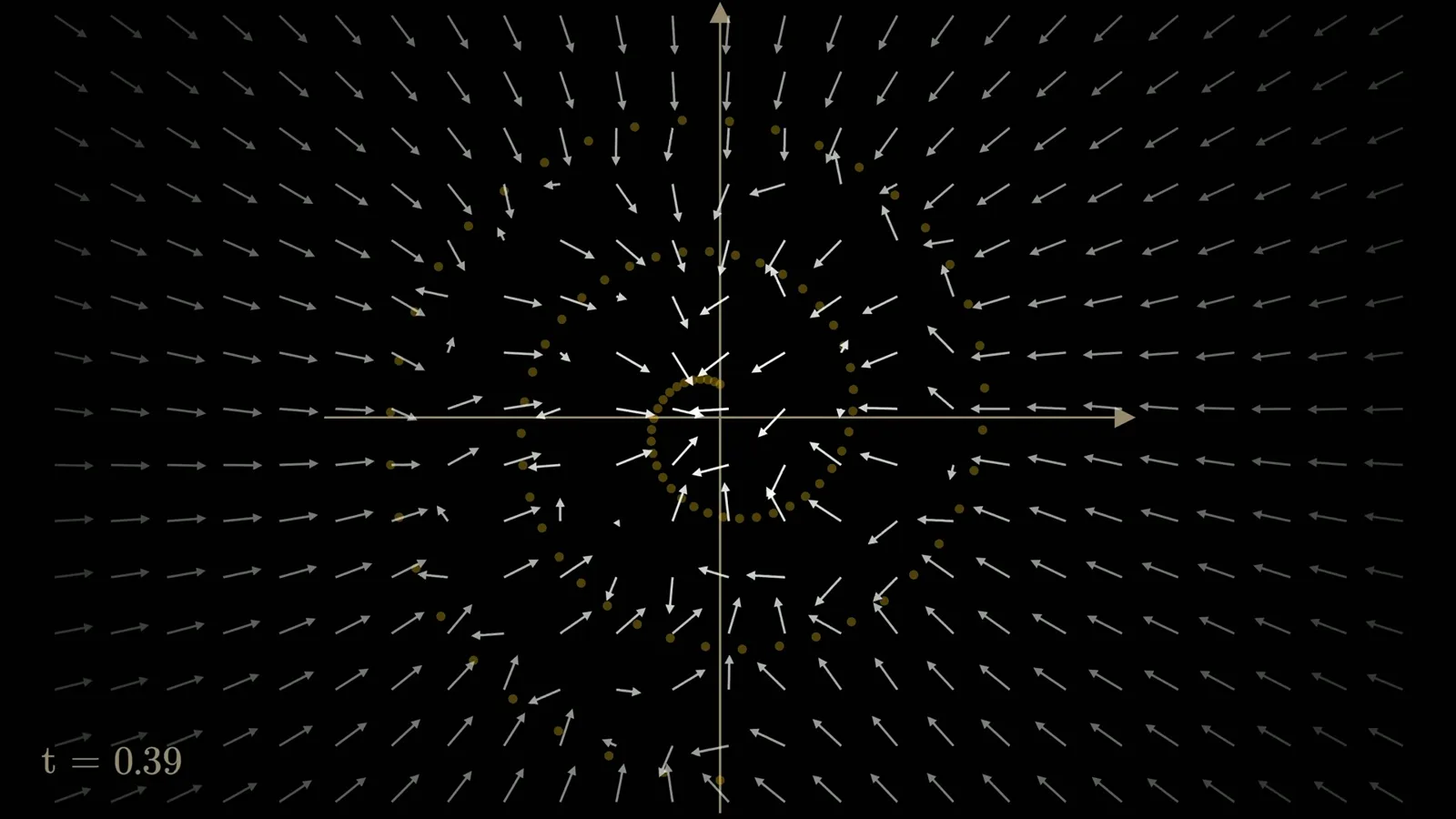
In DDPM sampling, start with a random point, move a little along the learned field, and add a scaled random step. Repeating this process gradually brings a cloud of points back to the spiral, with the random step decreasing as sampling proceeds.

If Welch removes the random step without changing the rest of the DDPM update, the points cluster near the mean rather than covering the spiral. He uses this to build intuition for blurry averaged images, while emphasizing that the two-dimensional analogy does not fully explain high-dimensional behavior.

The reverse transition can be approximated by a Gaussian distribution for sufficiently small steps. The model predicts its mean; adding appropriately scaled zero-mean noise samples the transition instead of always taking that mean. This explains the noise term in the stochastic DDPM procedure.

DDPM’s early drawback was computational cost: high-quality generation required many neural-network evaluations. Later work showed that a related deterministic process could generate high-quality samples without injecting noise at every step.

The stochastic process can be described by a stochastic differential equation. Using the Fokker–Planck connection, researchers derived an ordinary differential equation whose evolving probability distribution matches the stochastic one under the theoretical assumptions. Individual sample paths need not match.

The practical DDIM approach resembles DDPM but changes step scaling as well as omitting random additions. These smaller, differently scheduled steps follow the learned field more appropriately. It is not equivalent to deleting a line of noise code from the original DDPM sampler.

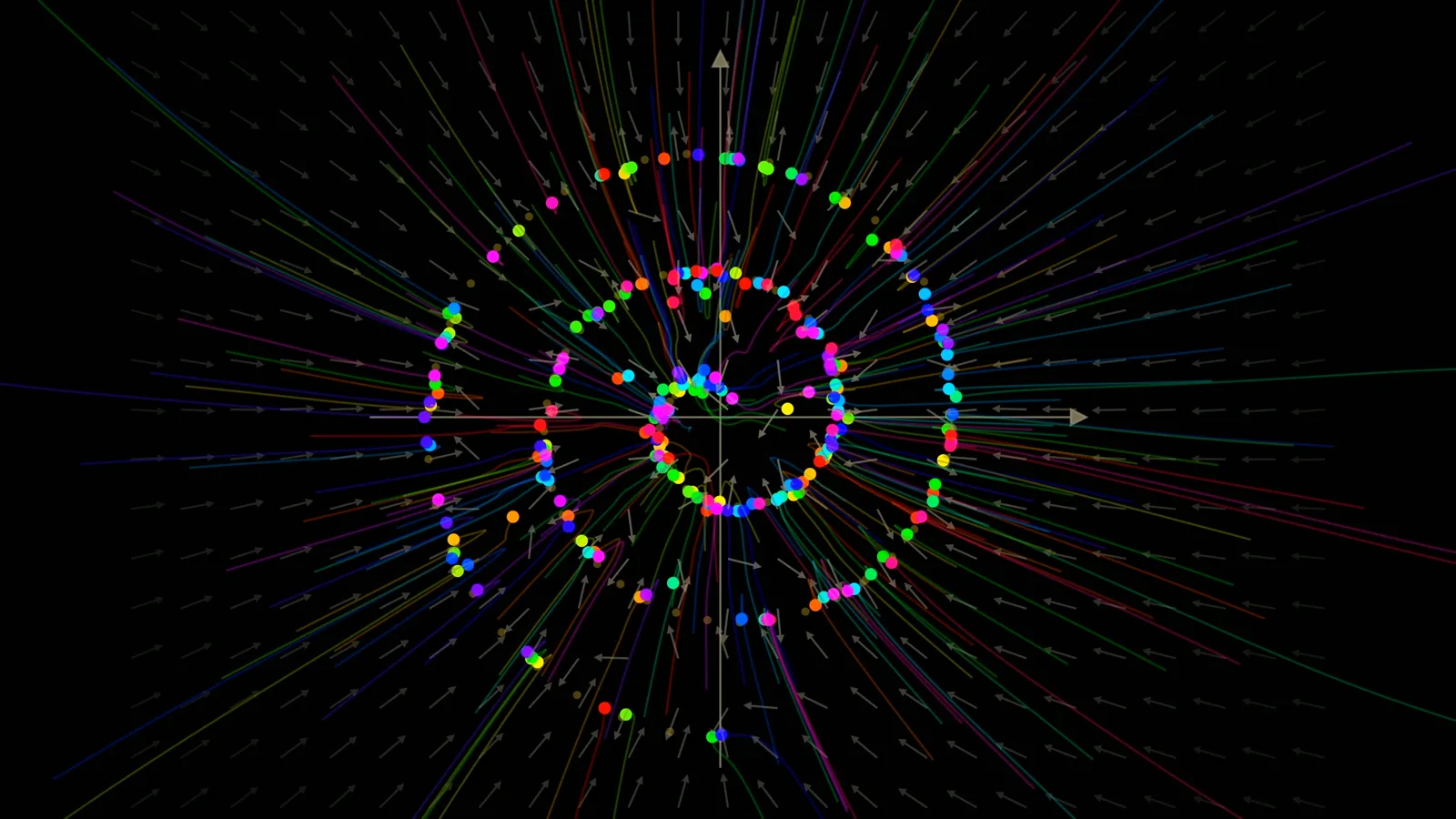
In the spiral example, DDIM’s deterministic paths cover the desired distribution; in the tree example it restores a coherent image. The same trained model can be sampled with fewer steps. The theoretical claim concerns distributions, not identical individual images.

Welch describes WAN’s approach as related to flow matching and then returns to text control. CLIP can represent a prompt, while diffusion can generate images; combining these ideas allows a text representation to influence the trajectory of generation.

DALL·E 2 used an approach called unCLIP to generate images guided by a shared image–text representation. One general way to steer a denoiser is conditioning: provide text information as an additional input while training on paired images and captions.

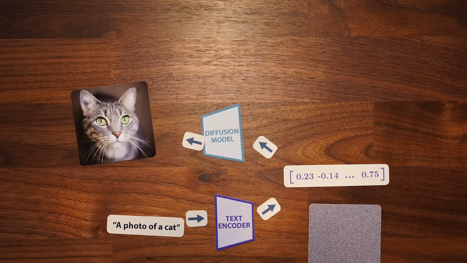
Conditioning can be implemented in different ways, including cross-attention or adding text representations to inputs. The description notes a detail for Stable Diffusion: its text conditioning uses an earlier sequence representation rather than simply the final 512-dimensional CLIP embedding.

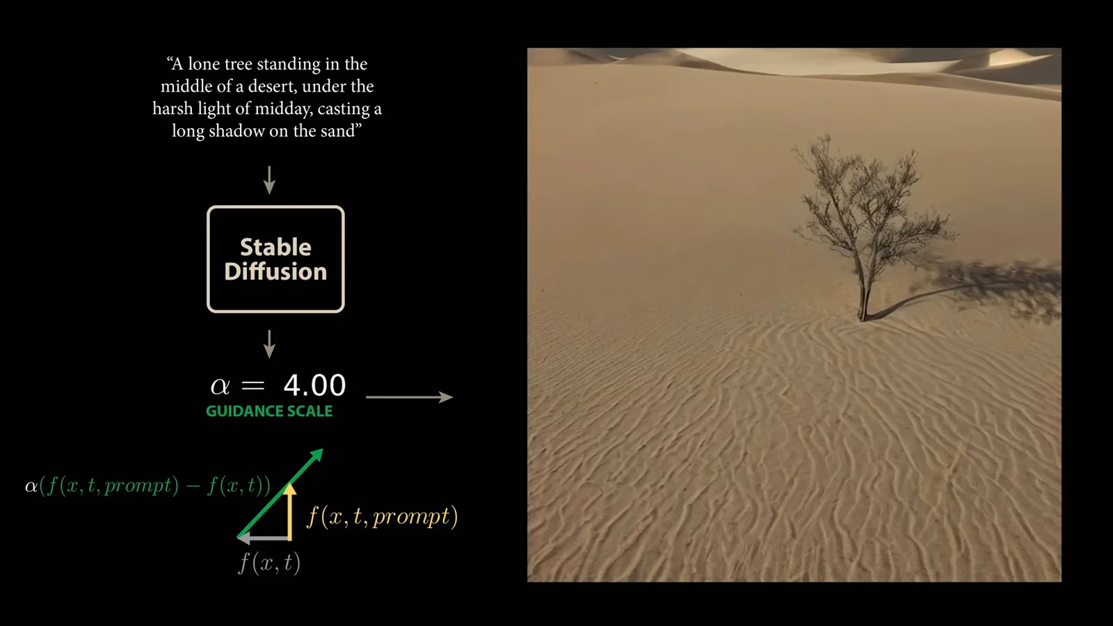
Conditioning alone may not strongly enforce every prompt detail. In Welch’s desert example, it can produce sand and a shadow without the requested tree. A toy spiral divided into people, dog and cat regions makes the problem visible: class-conditioned trajectories do not always reach the intended region.

Classifier-free guidance compares two predictions: one with the requested condition and one without it. During training, the condition is omitted for some examples, allowing the same network to produce both types of prediction.

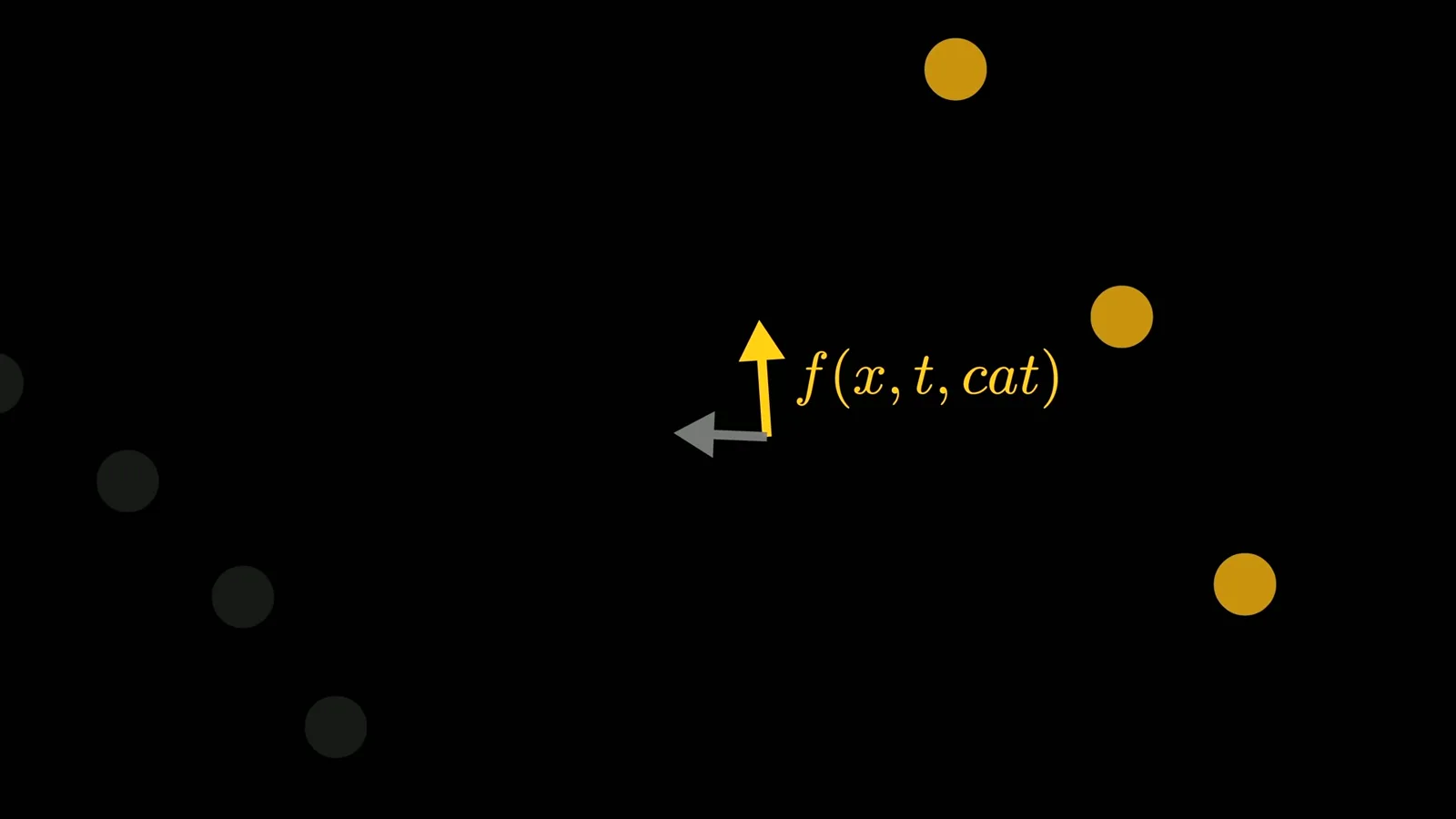
Subtract the unconditioned direction from the conditioned direction to isolate a component associated with the prompt, then scale that difference and combine it with the base prediction. Increasing guidance steers samples more strongly toward the requested class. Implementations use different scaling conventions.

In the toy dataset, guided cat and dog samples land more reliably in their respective regions. In the desert example, increasing guidance makes the tree appear and grow more detailed. Stronger guidance changes the result; the video does not claim unlimited guidance always improves it.

WAN also uses a negative prompt: instead of comparing against an empty condition, it uses a description of unwanted features and steers away from that direction. Welch notes examples such as extra fingers and backward walking, and shows that removing the negative prompt changes the generated scene.

The striking result is that several separately developed ideas fit together: a text encoder represents the prompt, and a learned diffusion or flow field shapes noise toward an image. Geometric intuitions that are easy to draw in two dimensions can help explain operations in much larger spaces.

The 3Blue1Brown host introduces Welch as the guest creator behind Welch Labs and explains that the guest series was commissioned during parental leave. Other planned videos explore statistical mechanics and the connection between modern art and group theory.