30 秒でわかる
Jane Street software engineer Tudor Brindus investigates jitter in a simple interprocess communication benchmark. He uses measurements and processor tracing to isolate sources of latency, then adjusts the operating system and application one step at a time. The exercise illustrates the tradeoffs between speed, determinism and stability, and why low-noise measurements help teams detect regressions.
- 1Start with the distributionThe virtualized ping-pong benchmark had a 637 ns median and outliers reaching roughly 16 microseconds. Its latency plots show why a single average is not enough.
- 2Move to bare metalRunning the same code without a virtual machine reduced median latency to 223 ns and cleared much of the noise.
- 3Trace rare eventsMagic Trace uses Intel Processor Trace to capture control flow around a slow round trip. The traces exposed network interrupts and later timer interrupts.
- 4Isolate cores and timer ticksCore isolation and reduced periodic ticks brought the median down further, while requiring explicit process placement.
- 5Trade speed for determinismDisabling turbo boost removed frequency-transition jitter in this test, but made the median slightly slower.
- 6Improve the spin loopAdding an x86 pause instruction reduced bad speculation from 8% to 1% and improved the median by 8 ns.
ポイント
- Latency-sensitive systems need to measure the distribution and tail of processing times, not just the median.
- Running the benchmark on bare metal removed substantial virtualization overhead and noise in this experiment.
- Processor tracing can reveal rare events that ordinary sampling profilers miss, including network and timer interrupts.
- Core isolation, reduced timer ticks and disabling turbo boost can improve determinism, with tradeoffs.
- A pause instruction in the spin loop reduced bad speculation and improved the benchmark.
- Hardware choice affects performance, but aggressive overclocking can compromise correctness.
チャプターごとに整えた全文を読む
Why jitter matters
Brindus introduces latency-sensitive market data and the need for predictable processing. He sets up a small interprocess benchmark.
I work on Jane Street’s ultra-low-latency trading team, where we deal with fast software, hardware and analysis tools. One recurring problem is jitter: variation in processing time. In trading, market data can arrive at around a gigabyte per second, depending on the exchange, and even data that is 10 microseconds stale can lead to bad trades.
Jane Street uses OCaml, which in the setup I describe has a fundamentally single-threaded runtime. Its async scheduler can dispatch blocking system calls to a thread pool, but parallel code execution requires multiple processes. That makes passing data between processes on the same machine an interesting case to study.
A ring-buffer ping-pong benchmark
Two processes exchange incrementing integers through ring buffers. Round-trip latency is measured on a Cascade Lake server.
A ring buffer can be thought of as an array of fixed-size cells: after reaching the end, the reader or writer wraps around to the beginning. We establish two buffers between two processes, one in each direction, and use them to play an endless game of ping-pong.
The pinger writes the integer 1; the ponger reads it, adds one and sends back 2. The pinger reads that, adds one and writes 3 to the next cell. The cycle continues around the buffers. I measure the time between the pinger writing a value and receiving the corresponding response.
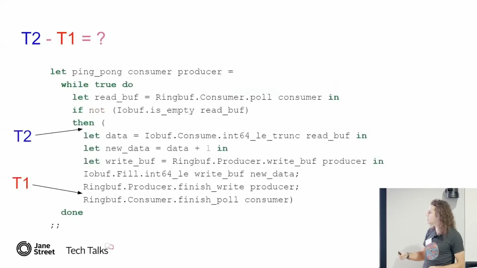
The benchmark runs on a second-generation Intel Cascade Lake server at 3.6 GHz. The initial setup is virtualized. Its median round-trip latency is 637 nanoseconds, but the jitter extends to roughly 16 microseconds: a large spread for such a small amount of work.
Virtual machines and bare metal
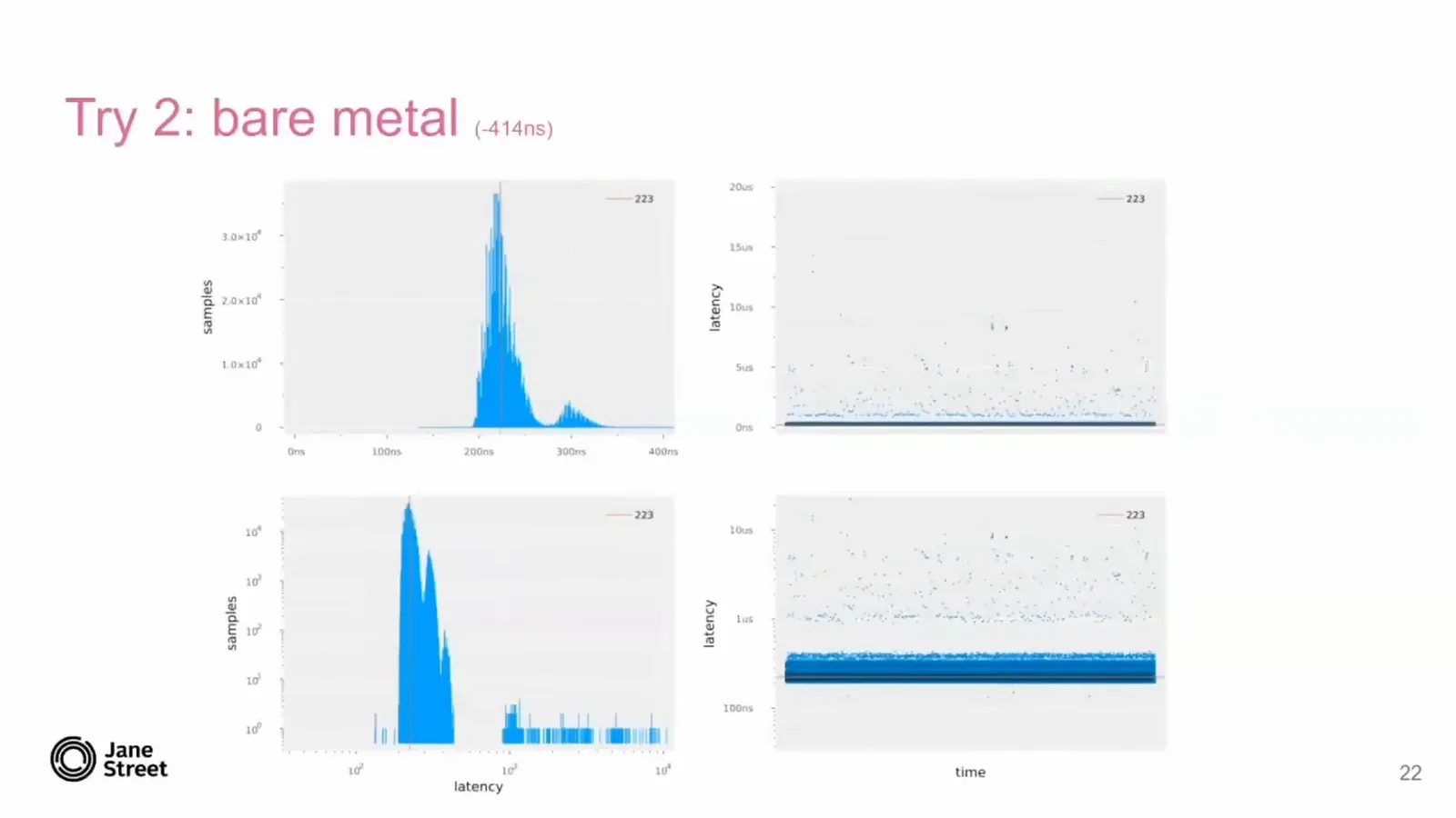
The initial latency distribution has a 637 ns median and a long tail. Running the same code on bare metal reduces the median to 223 ns.
The charts show histograms on the left and samples over time on the right. The upper plots use a linear scale; the lower ones use a logarithmic scale, which becomes more useful as the noise shrinks. The orange line marks the median.
A virtual machine might suffer from a noisy neighbor on the same physical host or other virtualization overhead. Rather than diagnose that complicated layer, I run the same code on bare metal. The median falls by 414 ns to 223 ns, and much of the noise disappears, although a concentration around one microsecond and longer tails remain.
A sampling profiler such as perf or VTune mostly reports that the processes are spinning while waiting for one another. That is accurate but does not explain the rare slow events. Our trading systems have a similar shape: they spend much of their time waiting for market data, and the interesting activity is infrequent.
Tracing rare latency events
Brindus explains Intel Processor Trace and Magic Trace. Capturing slow round trips reveals network interrupts in a program that does no networking.
Intel Processor Trace records control-flow transfers such as branches, calls and returns in compressed form. For conditional branches it can record taken or not taken as a bit; with the starting instruction pointer and a disassembler, the path can be reconstructed. A fixed-size circular trace buffer can be snapshotted when an interesting event occurs.
Jane Street built Magic Trace to decode and visualize this information. Its chart places call-stack depth on the vertical axis and time on the horizontal axis, allowing us to zoom in to a few nanoseconds of resolution and inspect what happened around an event.
Knowing the median, I define an interesting event as a round trip exceeding 300 ns. The trace shows spikes amid the normal exchange of integers. Zooming in reveals network activity in the kernel, despite the fact that this application only exchanges data through memory.
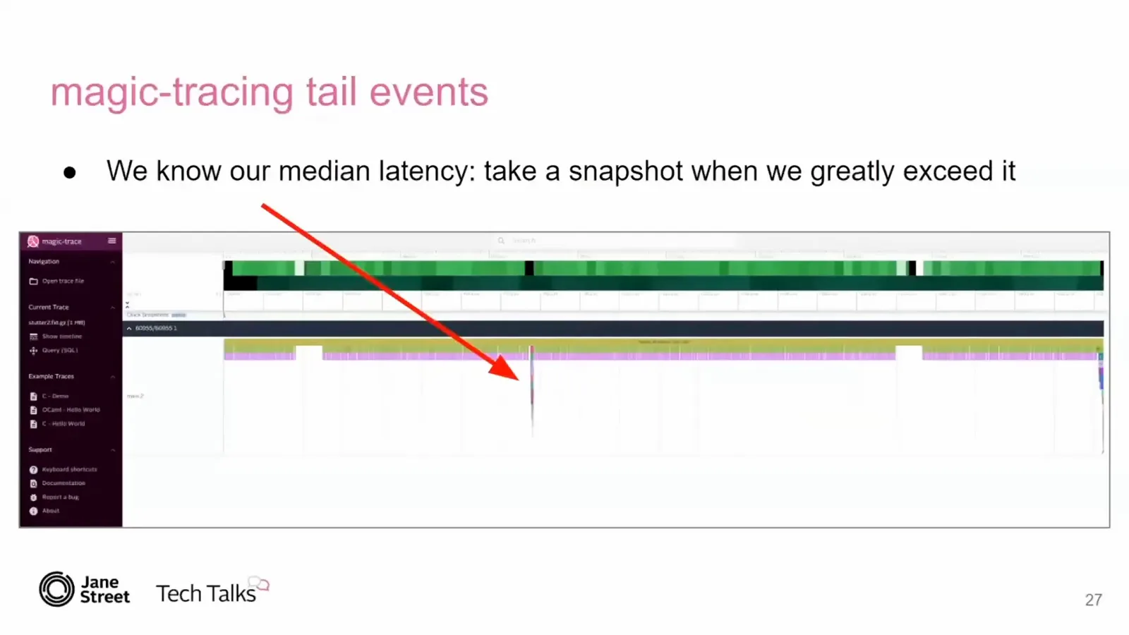
When a network card receives a packet, it interrupts a CPU so the kernel can dispatch it. Interrupts are normally distributed across cores for load balancing, which makes sense for heavy network traffic but can interrupt an application that has nothing to do with networking.
Isolating interrupts
Core isolation keeps network interrupts away from the benchmark, and reduced timer ticks remove another source of jitter. Each change is measured.
The Linux isolcpus parameter lets us set aside cores while leaving some available for network activity and remote access. The scheduler no longer places work on the isolated cores automatically, so we explicitly pin the pinger and ponger with taskset. After rebooting, network interrupts stay on other cores and the median drops another 29 ns to 194 ns.
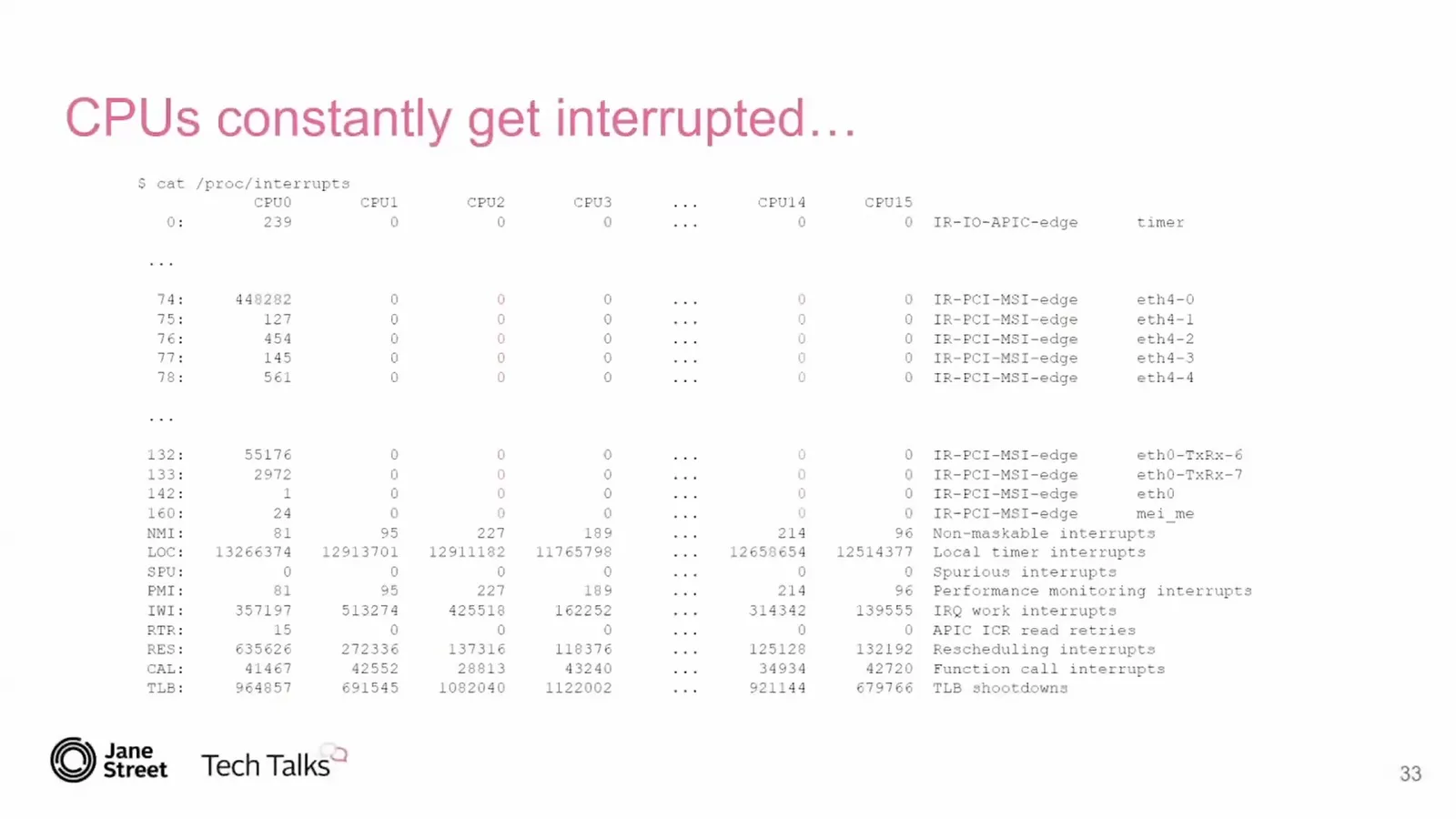
The one-microsecond tail is now more prominent. Magic Trace reveals an APIC timer interrupt, and /proc/interrupts shows how frequently local timer interrupts occur. The kernel traditionally uses these ticks to consider scheduling, update statistics and, on older CPUs, help manage frequency.
With one runnable process per isolated core, the nohz_full parameter can reduce these timer ticks. The kernel still needs some statistics updates, so the frequency can fall to about once a second rather than literally zero. This change saves another 24 ns and largely removes the one-microsecond mode, although longer tails remain.
At this point Magic Trace no longer shows an obvious interruption: the same instructions sometimes just take longer. That suggests a microarchitectural cause. One candidate is turbo boost, which changes CPU frequency dynamically within the processor’s power constraints.
Turbo boost and speculation
Frequency transitions and speculative execution introduce further variation. Brindus trades turbo speed for determinism and uses a pause instruction in the spin loop.
Our Cascade Lake server has a 3.6 GHz base frequency and can boost to 4.4 GHz through 31 possible P-states. Frequency transitions take time. I suspect the sawtooth pattern in the latency time series reflects transitions between nearby states, with one direction taking longer than the other; that is a hypothesis, not a confirmed explanation.
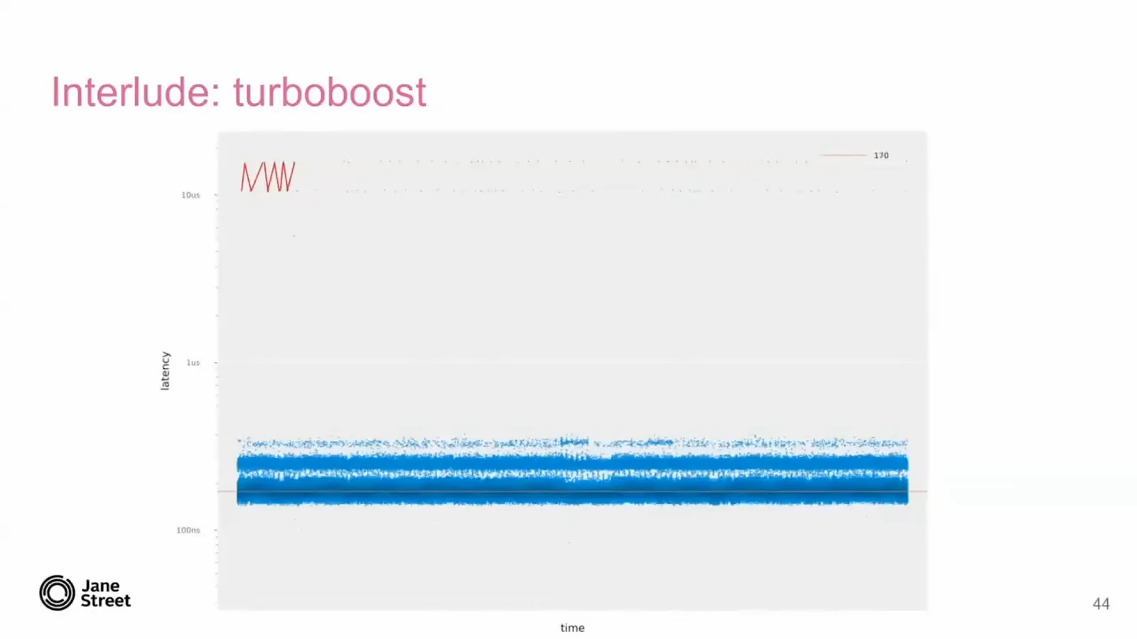
Turning off turbo boost removes that jitter, but the benchmark becomes one nanosecond slower. We have favored determinism over speed, running at 3.6 GHz rather than near 4.4 GHz. A workload doing more than incrementing a number would likely feel the frequency difference more strongly.
Three peaks remain in the logarithmic distribution. To understand another possible source, consider the gap between CPU speed and memory latency. A processor that must wait for a dereferenced memory operand would stall badly, so designers use techniques including speculative execution to hide that delay.
In our polling loop, the ring buffer is empty most of the time. The CPU learns to predict that another load will also find no data, loops back speculatively and issues further loads. Eventually a load does contain data; the processor must discard the incorrect speculative work and restore the appropriate state.
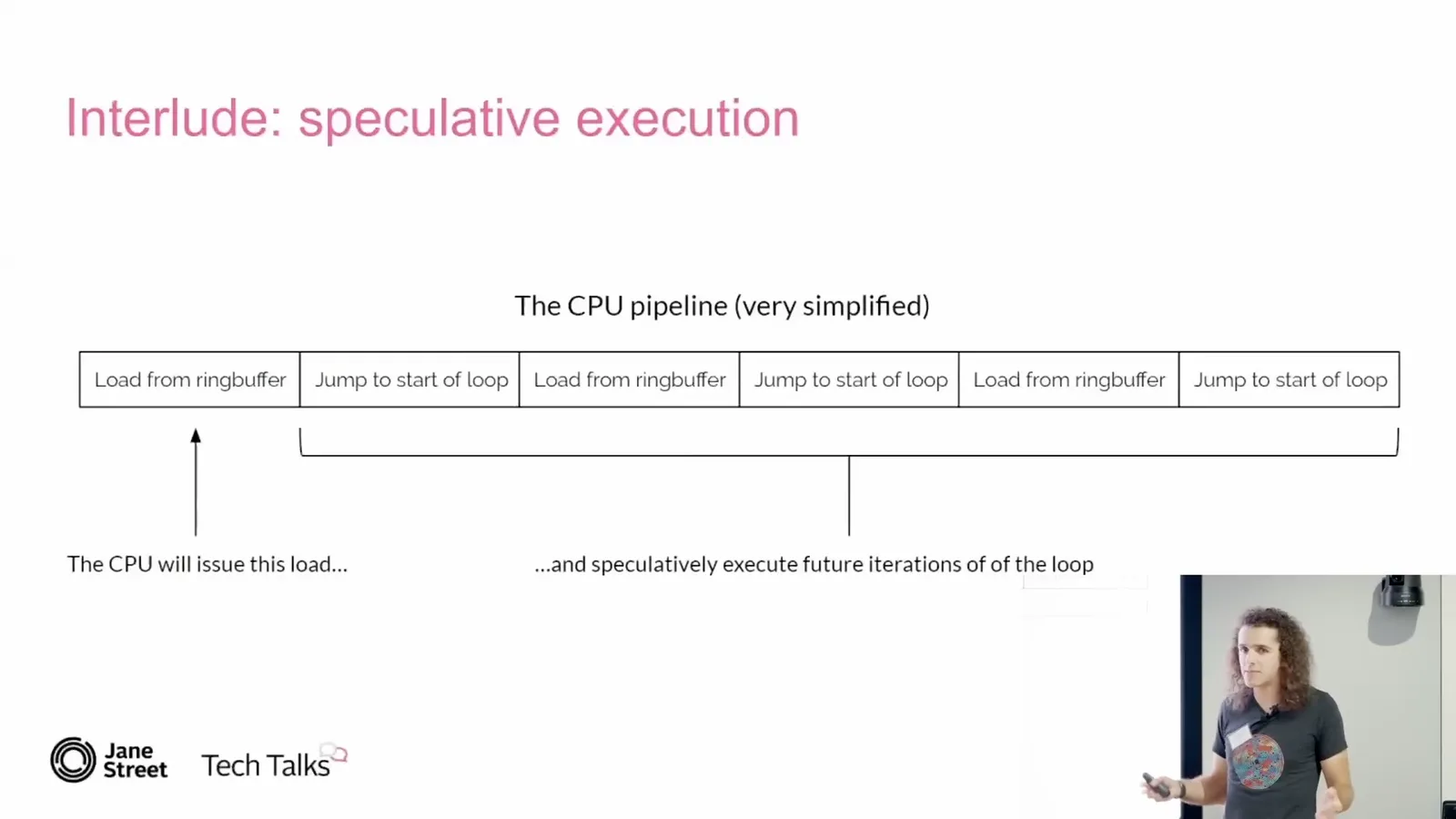
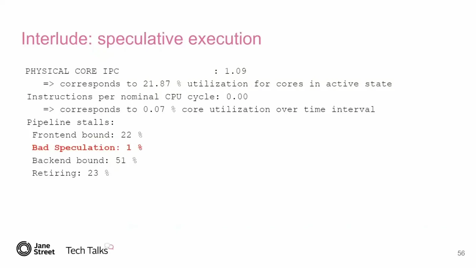
Intel’s PCM tool attributes 8% of the observed pipeline breakdown to bad speculation. Other categories have larger percentages, but I cite Intel’s optimization guidance that bad speculation above 1% deserves attention. The polling loop resembles a spin lock, a case the x86 pause instruction is designed to help.
The pause instruction hints that the processor is in a spin-wait loop and helps avoid the penalty associated with exiting it. We ask our compiler developers for an OCaml intrinsic that emits it. With that one-line change, bad speculation falls from 8% to 1%, and median latency improves by another 8 ns.
The three peaks largely collapse into one, though some samples remain in slower bands that I cannot explain. On the original hardware, we have gone from 637 ns with substantial jitter to 163 ns with much less jitter. That is a substantial improvement for a very small code change.
Hardware, tradeoffs and measurement
An overclocked server improves the benchmark but proves unstable under real workloads. Brindus discusses virtual machines, containers and the value of continuously monitoring tails.
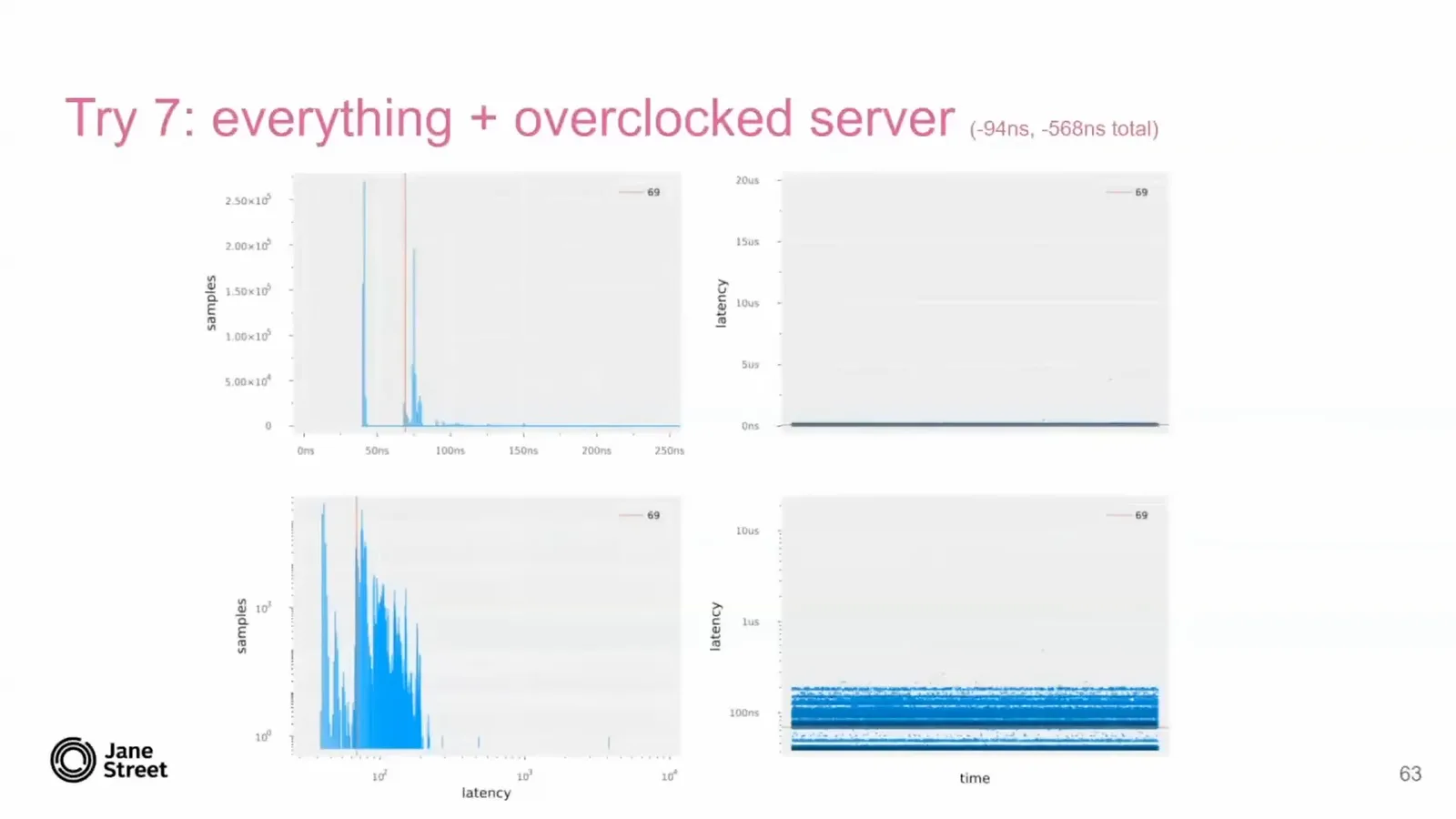
What if we use faster memory and an overclocked CPU? The benchmark improves by another 94 ns, to a 69 ns median. But there is an important qualification: when we tried real trading systems on this machine, it died halfway through a test with memory corruption. Aggressive overclocking can make the result fast and wrong.
If performance and determinism matter, consider the cost of virtualization and understand the environment you are using. In response to a question, I note that AWS is a reputable provider but virtual machines can still have jitter; it also offers bare-metal instances. Lower-end providers may oversubscribe their hardware.
Asked about Docker, I distinguish containers on bare metal from a hypervisor-based virtual machine. Docker uses kernel namespaces, and cgroup accounting can make kernel interactions moderately slower. For code that avoids system calls, I would not expect the same kind of additional virtualization jitter.
Understanding the architecture can unlock considerable performance, and hardware choice matters. Most of all, keep measuring. When a system already has noisy tails, a regression can hide in the noise and become much worse before anyone notices.
When median and p99 latency are close, a new regression that sends p99 sharply upward is much easier to detect during testing. That is a more stable position from which to maintain a system when determinism matters.
同じチャンネルの記事
 1:48:29EN
 1:36:37EN
 1:05:45EN
 1:25:00EN
 1:16:29EN
 27:39EN