Echoes of Fourier: From Sound Waves to Fast Convolution

I want to explore the relationship between echoes and the Fourier transform. To work with sound mathematically, start by treating a recording as a function of time: its value describes the pressure at each moment. The waveform is made of oscillations at many frequencies, combined in different ways.

For computation, we replace continuous time with discrete samples. At 44,100 samples per second, one sample represents 1/44,100 of a second. The sound is therefore a function of discrete time, or a vector of sample values.

Before processing it, we need complex numbers. A complex number has real and imaginary parts and can be represented by a point in the complex plane. Polar coordinates describe that point by its distance from zero and its angle measured from the real axis.

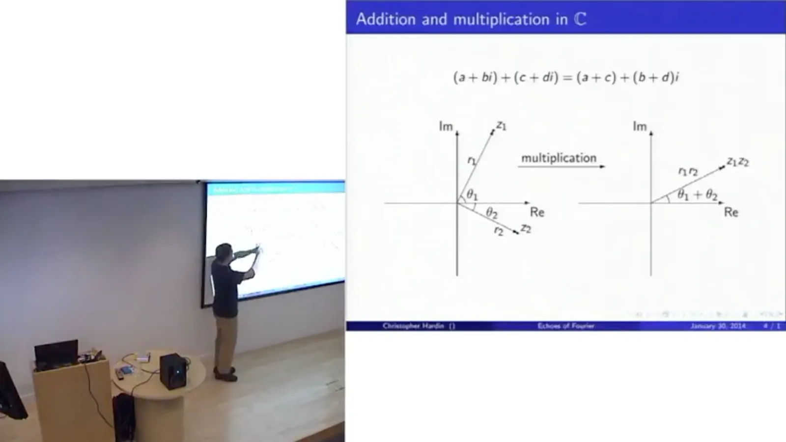
Addition combines real and imaginary parts separately. Multiplication is easier to visualize in polar form: multiply the two radii and add the angles. Angles are measured counterclockwise, so a clockwise angle is negative.

We can extend functions such as the exponential, sine, and cosine to complex inputs using their power series. Substituting an imaginary argument into the exponential series separates its real and imaginary terms into the series for cosine and sine.

That gives Euler's formula, e^(iθ) = cos θ + i sin θ. Its absolute value is one, so as θ increases, the point travels around the unit circle. For example, e^(iπ/2) = i and e^(iπ) = −1.

Circular motion is a particularly natural form of periodic motion. A weight on a spring traces a circle in a suitable position-and-velocity phase space; sine and cosine can be thought of as its projections. This makes complex exponentials useful building blocks for periodic signals.

Rather than separately decomposing a signal into sines and cosines, we can use complex sinusoids at different frequencies. Positive frequency corresponds to counterclockwise motion around the circle, and negative frequency to clockwise motion.

We will also make time finite: there are N distinct sample positions, and after N the index wraps around to zero. A sound is then a vector in the N-dimensional complex space C^N, equivalently a function on the sample indices 0 through N−1.

The complex sinusoid exp(2πit/N) completes one revolution as t runs through the sample interval. Adding an integer frequency ω in the exponent produces ω revolutions; a negative ω reverses the direction. Think of this expression as a wave of frequency ω.

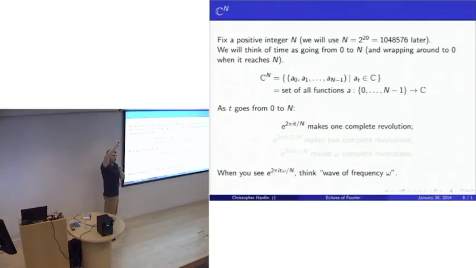
The example sound is real-valued, although we are working in a complex vector space. The important theorem is that any such vector can be expressed as a sum of complex sinusoids, each multiplied by a coefficient. In linear algebra language, those sinusoids form a basis for C^N.

The magnitude of a coefficient tells us how much of its frequency is present. Its angle, or phase, carries timing information. Together these coefficients describe the same sound in a different coordinate system.

Why do the waves form a basis? With the complex inner product, which conjugates one factor, the inner product of two waves involves a sinusoid at the difference of their frequencies. For distinct frequency indices, its values are evenly distributed around the unit circle and sum to zero.

The waves are therefore mutually orthogonal. N nonzero perpendicular vectors in an N-dimensional space are linearly independent and form a basis. When the frequencies are the same, the difference is zero, so the sum does not vanish.

The coefficients can be recovered using a formula that resembles the reconstruction formula, but with the exponent's sign reversed and a normalization factor placed according to convention. This follows from taking inner products with the orthogonal basis vectors.

The discrete Fourier transform maps the time-domain samples to those frequency coefficients; the inverse transform maps the coefficients back to the samples. The transform is a change of basis, not a loss of the original signal.

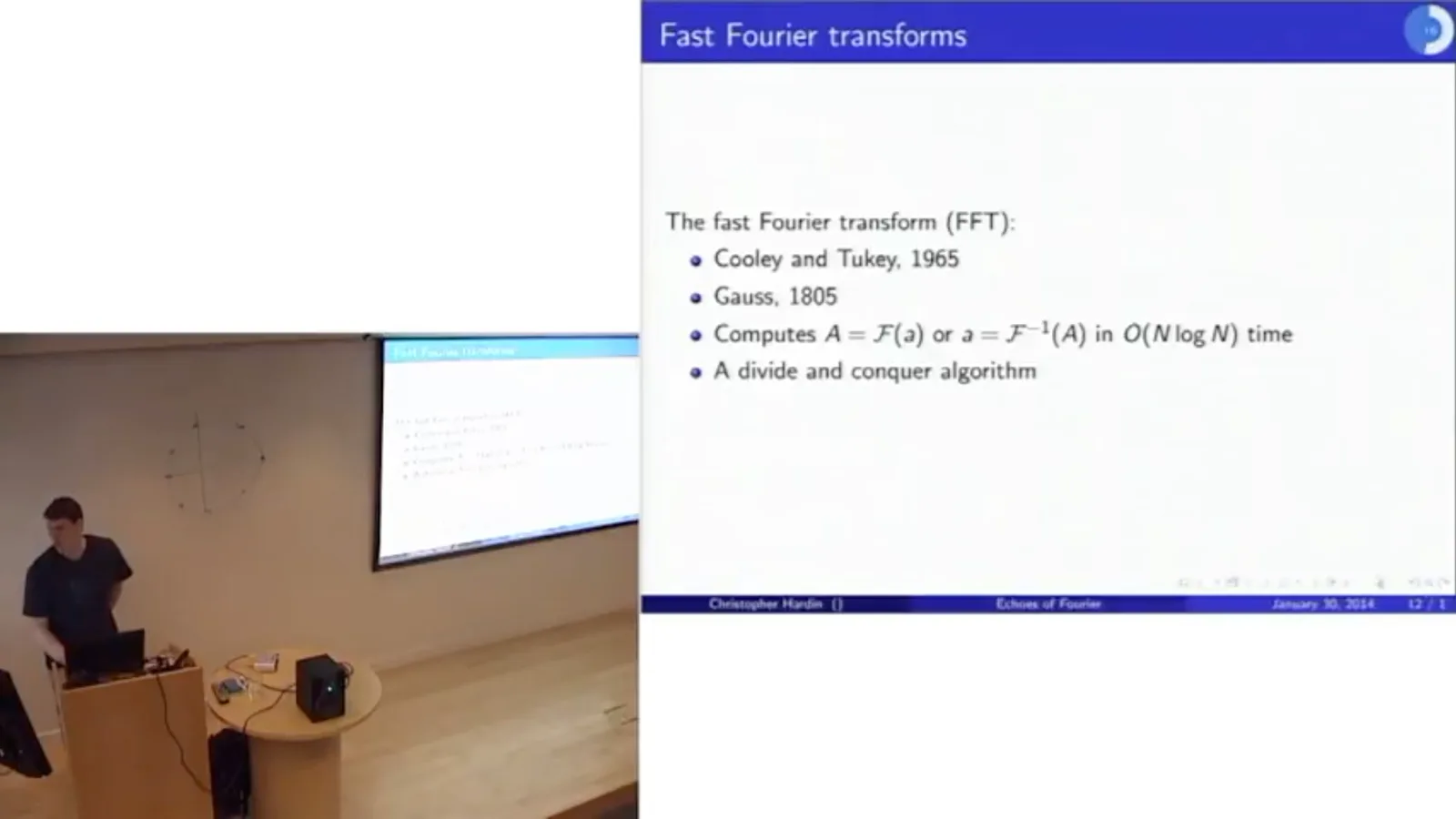
The fast Fourier transform, or FFT, is an algorithm for computing the discrete transform and its inverse in O(N log N) time. Cooley and Tukey published a version in 1965; Hardin notes an earlier version by Gauss. Its divide-and-conquer approach transforms the even and odd indexed samples separately and combines the results.

In an Octave demonstration, I transform the song and plot the magnitudes of its frequency coefficients. For a real-valued signal, the high-frequency side mirrors the low-frequency side: a rotation of seven-eighths of a turn per sample is indistinguishable at the samples from a negative one-eighth turn.

The low-frequency plot has many peaks, which may reflect resonances of the instrument or the recording space. The magnitudes are only part of the information; each coefficient also has a phase. A separate phase plot is much harder to interpret by eye.

As a simple filter, keep only frequencies from 300 to 400 hertz and set the others to zero. The frequency bin must be converted from cycles over the whole recording to cycles per second. We also retain the corresponding negative-frequency components so the reconstructed signal remains real.

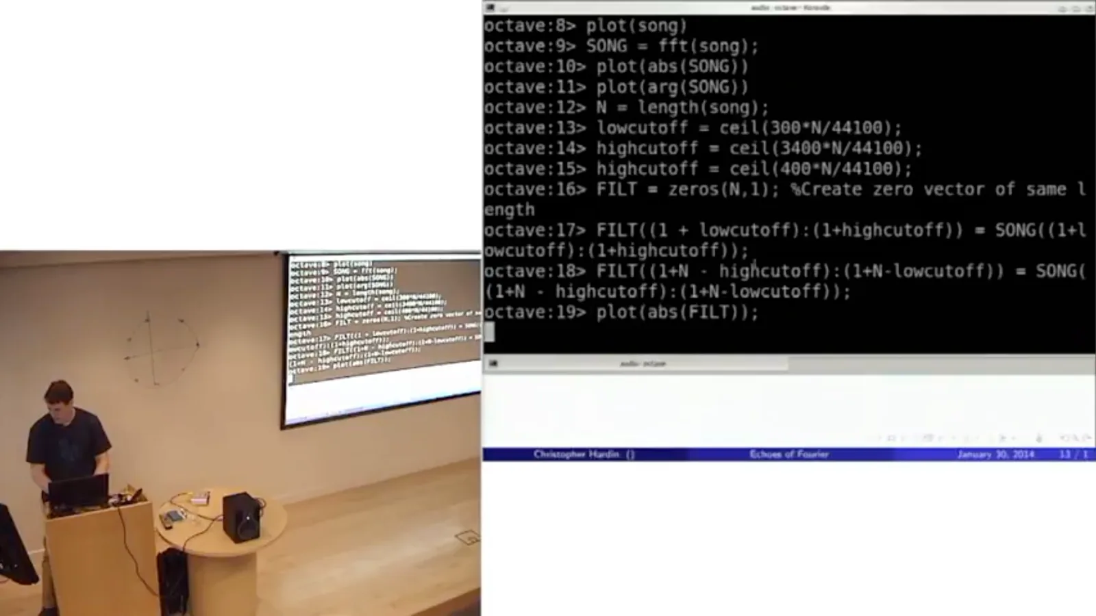
After the inverse transform, the filtered recording sounds markedly different. The frequency representation lets us select a band directly, then turn the result back into sound. Small imaginary remnants can arise from numerical roundoff and can be discarded for this real-valued signal.

Taking a transform and its inverse returns almost the original recording: the remaining differences are tiny floating-point errors. This round trip is a useful practical check before using the same machinery for more interesting processing.

Now consider an echo. If a sound is made in a space, reflections arrive at different delays and strengths. The pattern of those delayed responses describes how the space changes an arbitrary recording; individual reflections can preserve or reverse sign depending on the boundary.

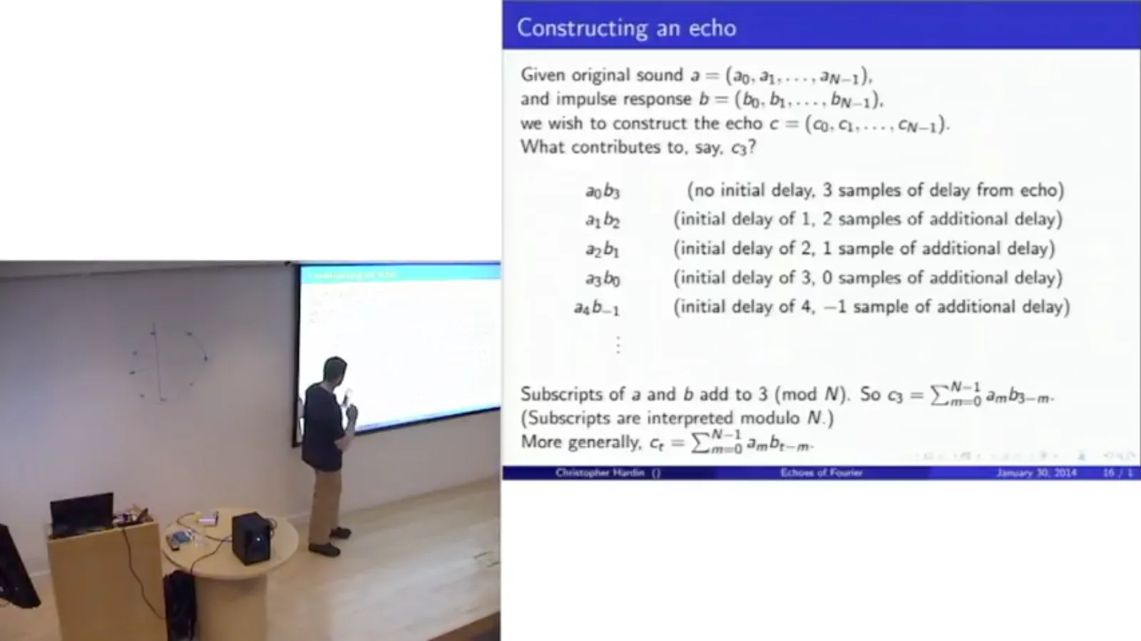
Call the original sound a and the echo pattern, or impulse response, b. To construct the output c at sample 3, add contributions such as a₀b₃, a₁b₂, a₂b₁, and a₃b₀: each combines an original sample with the delay needed to reach sample 3.

In our circular model the indices are interpreted modulo N. In general cₜ = Σₘ aₘbₜ₋ₘ, with m running over the N samples. This operation is convolution, written a * b. It describes what a recording would sound like after passing through the space represented by b.

For a simple example, if the impulse response contains a one and then a half at a later delay, the output contains the original signal plus a delayed copy at half its amplitude. Padding the vectors with enough zeros keeps the circular wraparound from interfering with the desired result.

The impulse response can be measured. A signal consisting of a single one followed by zeros is a sharp pop; convolving it with b gives b itself. Record a balloon pop or an electric spark in a space and the resulting sound approximates the space's impulse response, including its later reflections.

The direct convolution formula takes N multiplications for each output sample, or roughly N² for all of them. At a million samples that becomes expensive. The convolution theorem gives us a much faster route.

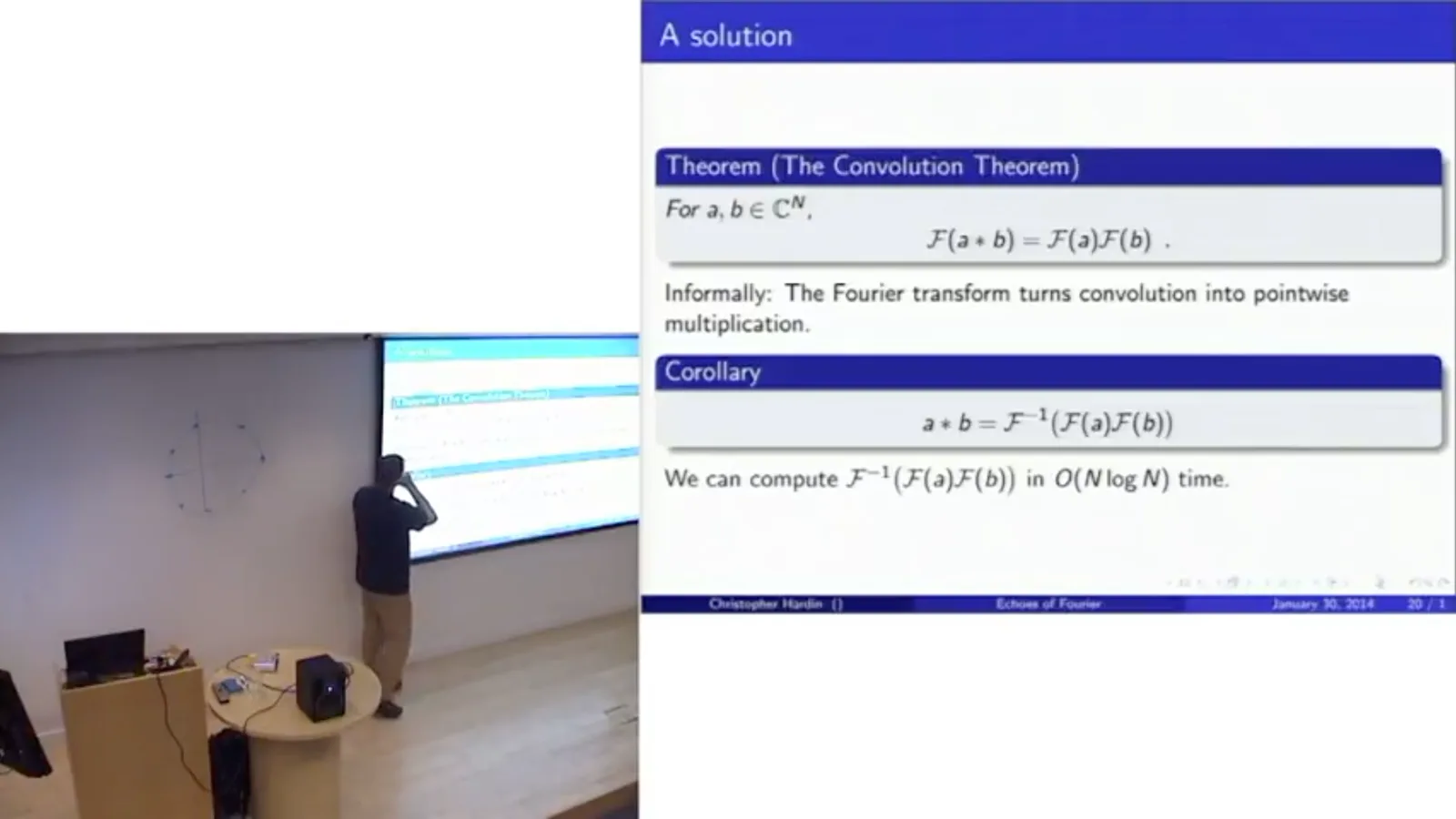
The theorem says that the Fourier transform of a convolution equals the pointwise product of the two Fourier transforms: F(a * b) = F(a)F(b). Thus a * b = F⁻¹(F(a)F(b)). The FFTs cost O(N log N), the multiplication costs O(N), and the whole computation is O(N log N).

The proof is an exercise in rearranging the sums and using the definitions of the transform and convolution. The significance is practical: an operation involving many delayed copies in time becomes ordinary pointwise multiplication in frequency.

For a real example, I use a recording of an impulse response made in Santa Lucia, a church in Italy. The sharp pop and the subsequent decaying reflections capture the acoustic response of that space. I select one channel of the stereo recording for the demonstration.

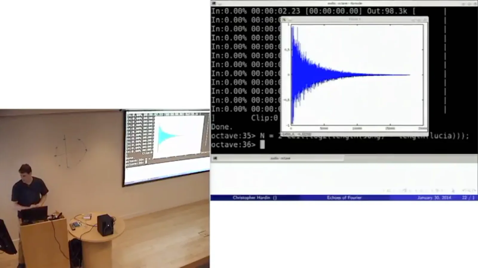
To apply it to the song, pad both signals with zeros to a suitable power-of-two length at least as large as the sum of their lengths. Transform each, multiply the results pointwise, and inverse-transform. The padding prevents the end of the convolution from wrapping into its beginning.

Roundoff can leave tiny imaginary components, so I take the real part. The output may also exceed the permitted playback range of −1 to 1; rescaling prevents clipping. Comparing the original with the result makes the artificially added reverberation audible.

A measured impulse response lets us bring the acoustics of a real place to another recording. But we can also make impulse responses for spaces that do not exist. I simulate a hallway two meters by three meters by thirty meters with very reflective walls.

The synthetic hallway response is processed in the same way: zero-pad, transform, multiply, inverse-transform, and rescale. The resulting recording sounds as if it were played in that imaginary hallway, with a much stronger, more distinctive reverberation.

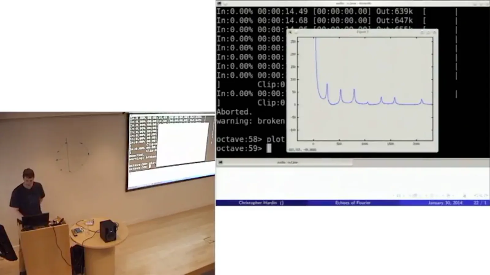
The Fourier transform of the hallway's impulse response shows resonance peaks. The first prominent peak corresponds to approximately 10.977 hertz. Using the speed of sound of about 331 meters per second gives a wavelength of roughly 30 meters, consistent with the simulated hallway's length.

The simulation works for rectangular solids by using a mirror-image construction. Imagine the walls as mirrors and the sound source as a light: repeated reflections produce an infinite three-dimensional lattice of image sources. Each image represents a possible reflected path.

The walls in this example reflect 99.9% of the sound. More reflections attenuate a path, as does greater distance. To build a finite impulse response, sum the appropriately delayed and attenuated contributions from image sources within a chosen range of travel times.

For a subtler example, simulate a three-by-three-by-three-meter room whose walls reflect 90% of the incident sound. Convolving a different recording with this response gives it the character of that smaller, more absorptive space.

A question asks whether convolution can be reversed. In the frequency domain, deconvolution means division by the response's Fourier coefficients. If any coefficient is zero, an exact inverse does not exist; coefficients close to zero can make the inverse enormous and numerically unstable.

The same ideas extend to two dimensions. For a grayscale image, transform each row and then each column. Convolving an image with a Gaussian-like bump blurs it; trying to recover the original by deconvolution is difficult for the same stability reasons. Sharpening can approximate the result without perfectly recovering the lost detail.

Digital room correction uses an approximate inverse of a room's impulse response. A sound system can apply that correction before playback; the room then adds its own response, leaving a better overall result. The inverse is approximate because perfect cancellation is generally impractical.

I tried isolating the first part of an impulse response, which should contain the direct sound before reflections, and deconvolving by it exactly. The result worked badly. An approximate inverse might be more useful when cleaning up an imperfect impulse-response measurement.

In practice, one can measure a room with a swept-frequency signal instead of a very sharp pop, then undo the known sweep mathematically. Spreading the energy over time helps avoid driving the microphone into nonlinear behavior, which would undermine the linear convolution model.