En 30 secondes
3Blue1Brown builds an intuition for the Laplace transform from complex exponentials, then visualizes the integral and explains analytic continuation. A cosine example shows how poles reveal oscillatory pieces and connects the result to Fourier analysis.
- 1Decompose motion into exponentialsA cosine is the sum of two counter-rotating complex exponentials, each scaled by one half.
- 2The defining integralMultiply a time function by e^(−st), then integrate from zero to infinity where the integral converges.
- 3Analytic continuationThe extended function can reveal poles even outside the region where the original integral exists.
- 4Exponentials become polesThe transform of e^(at) is 1/(s−a) in its region of convergence.
- 5The cosine exampleLinearity yields two terms with poles at i and −i; for frequency ω the compact answer is s/(s²+ω²).
À retenir
- Complex exponentials encode oscillation and growth or decay through the imaginary and real parts of their exponents.
- The Laplace transform integrates f(t)e^(−st) from zero to infinity wherever that integral converges.
- An exponential e^(at) transforms to 1/(s−a), with a pole at a in its analytic continuation.
- Linearity turns sums of exponentials into sums of transformed terms, exposing their poles.
- Analytic continuation extends a complex function beyond the region where its original integral converges, but does not make the divergent integral converge.
- The cosine transform has poles at ±iω and is closely related to Fourier analysis.
Lire le texte remanié, chapitre par chapitre
Looking inside the transform
The lesson seeks intuition for a tool used in differential equations. Complex exponentials give the central language.
You can learn to drive a car without understanding its engine, and you can learn to use the Laplace transform without understanding its inner workings. Both kinds of knowledge have value. Here the goal is to open the hood and see the mathematics that makes the tool useful.
Start with e^(st), where t is time and s may be complex. The imaginary part of s makes the output rotate in the complex plane; a negative real part makes its magnitude decay, while a positive real part makes it grow.
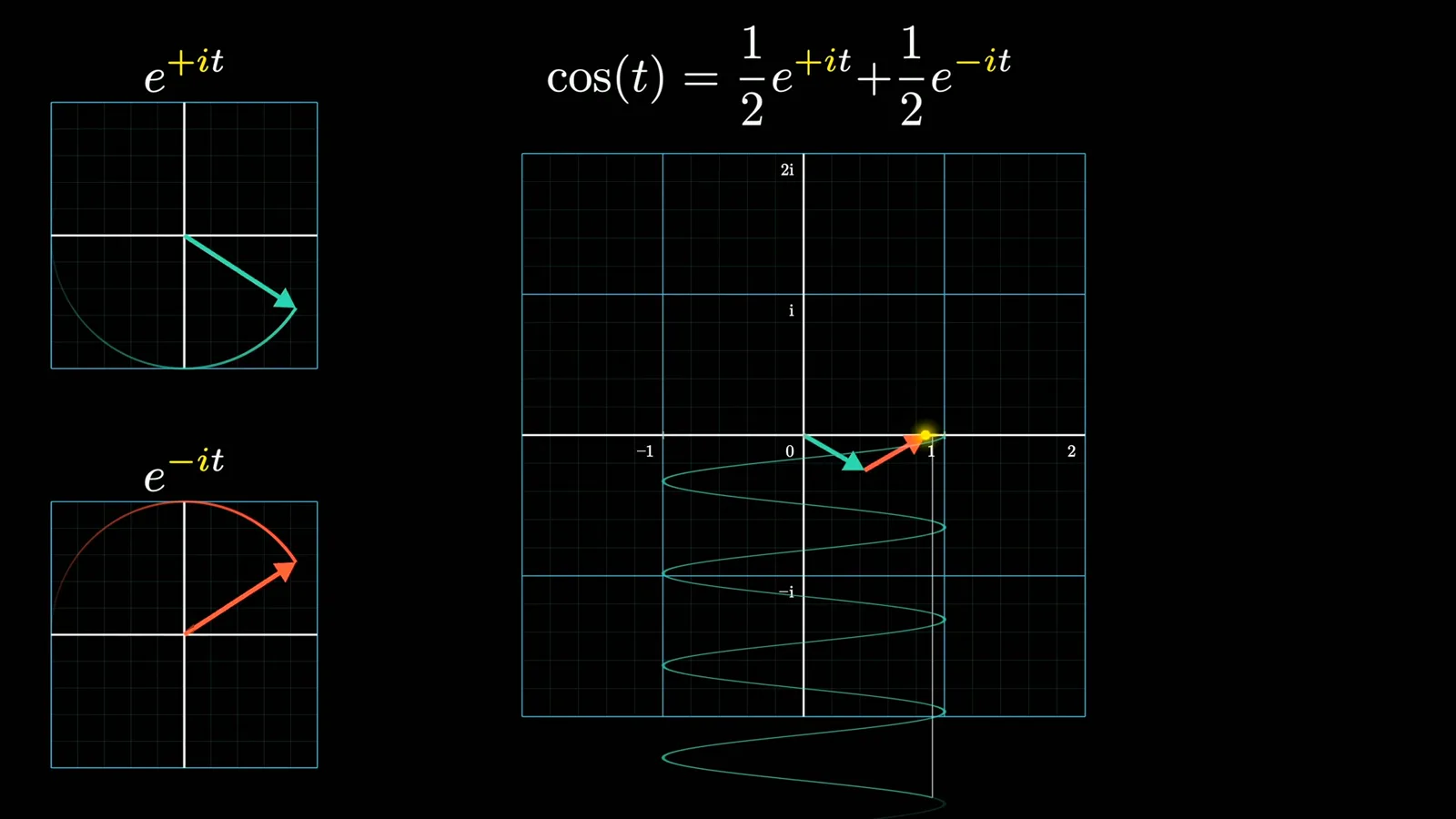
Many functions arising in physics can be expressed as combinations of exponentials. A familiar example is cos(t) = ½e^(it) + ½e^(−it). The two vectors rotate in opposite directions, their imaginary parts cancel, and their sum oscillates on the real axis.
A driven spring provides a more complicated example: its solution can involve two exponentially decaying oscillatory pieces and two pieces that follow the external force. We want a machine that reveals the exponents and coefficients hiding inside a function.
Exponentials are useful because differentiating e^(st) amounts to multiplying it by s. A tool that exposes exponential pieces can therefore help turn differential equations into algebra. Engineers call the complex plane of possible exponents the s-plane.
Each point of the s-plane represents an entire exponential function. Greater imaginary magnitude means faster oscillation; moving left or right changes decay or growth. A transform takes a whole function as input and returns another function, conventionally written F(s).
The transform as a detector
The transform maps a time function to a function on the complex s-plane. Its poles can expose exponential pieces.
For a function that is a sum of exponentials, plotting the transform over the s-plane produces sharp spikes called poles at the corresponding exponent values. The poles offer a way to discover the components even if we did not know the decomposition beforehand.
The definition has two steps: multiply f(t) by e^(−st), then integrate the result from t = 0 to infinity. The complex parameter s is the input to the new function. We can imagine moving it around the plane to probe which exponentials align with f.
For cosine, substitute its two exponentials. Multiplying e^(it) by e^(−st) gives e^((i−s)t). At s = i that component becomes the constant 1 rather than spiraling or decaying. Integrating a constant indefinitely diverges, hinting at the spike over that special value.
That intuition needs care because the integrand is complex-valued and the infinite integral does not converge everywhere. To see what is happening, first ignore f(t) and integrate e^(−st). For real s = 1, the integral is 1: the area under the exponential curve.
Visualizing the integral
The integral can be understood as a sum of average values over unit intervals. For complex values, those averages add as vectors.
For positive real s, horizontal scaling gives area 1/s. As s approaches zero from the positive side, the tail decays more slowly and the area grows without bound. To extend this intuition to complex values, think in terms of averages instead of area.
On a unit interval, the integral equals the average value of the function over that interval. Split the positive time axis into intervals of length one, take each average and add them. Their limiting sum, when it exists, gives the integral from zero to infinity.
For complex s, e^(−st) traces a path in the complex plane. The average over each unit interval is itself a complex number, represented by an arrow. Add the arrows tip to tail; if the resulting sequence converges, its limit is the value of the integral.
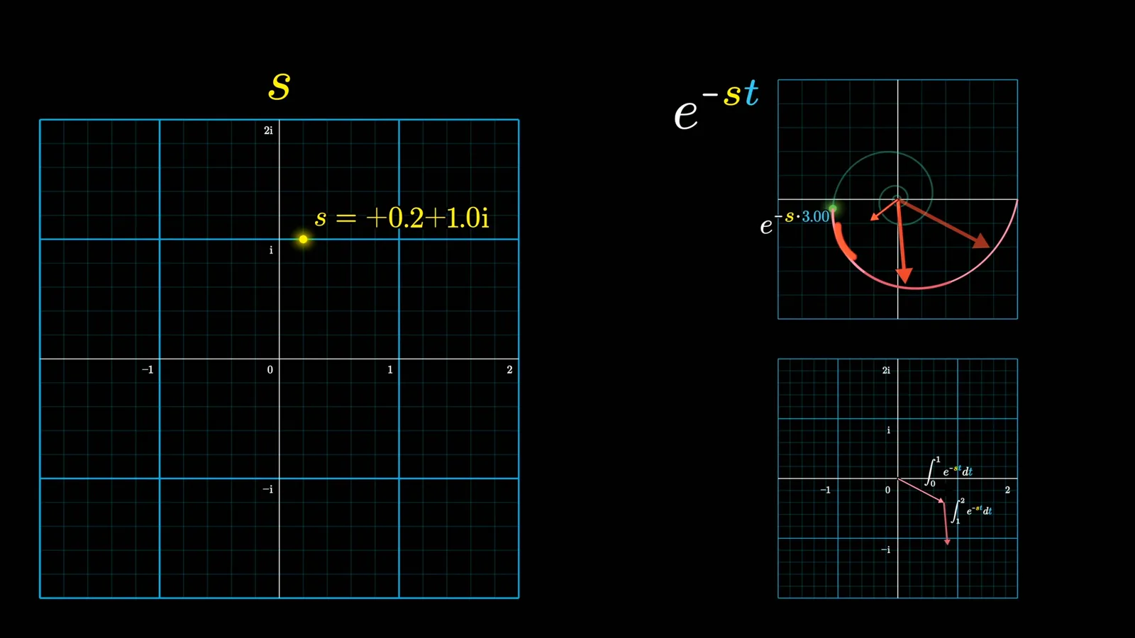
At s = 1, the arrows lie on the real line and sum to 1, agreeing with the area calculation. Moving s toward zero increases the result. Changing its imaginary part introduces rotation and cancellation among the arrows, reducing the output magnitude in the illustrated cases.
Plot the magnitude of that limiting vector as height above each s and use color to represent its direction. The plot rises sharply near zero. Slow decay and little cancellation make the value large, while faster oscillation creates more cancellation.
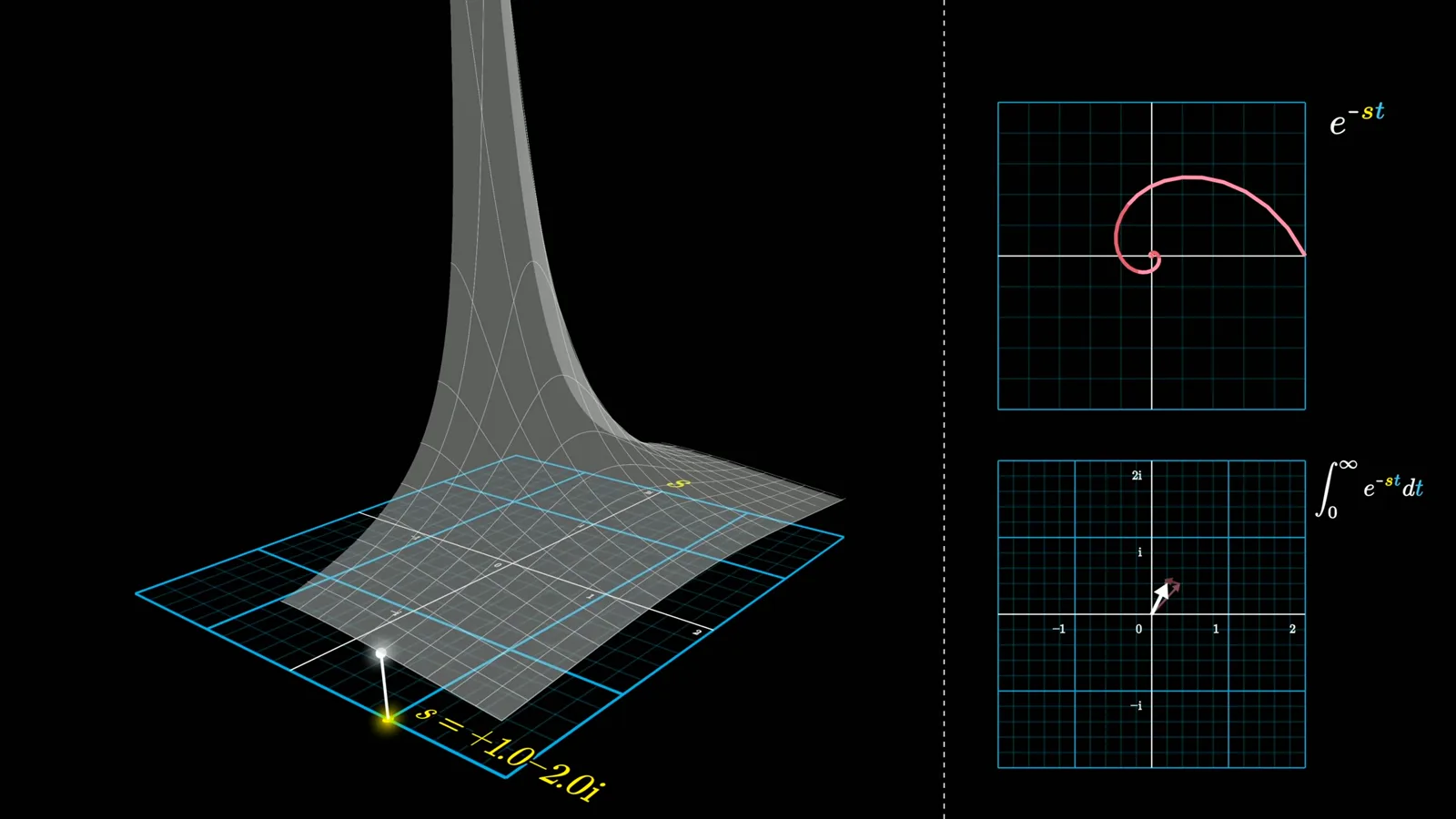
Convergence and continuation
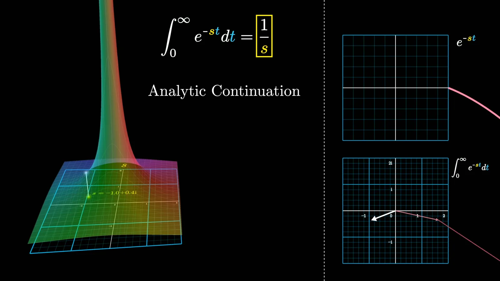
The integral for e^(−st) converges only on the right half-plane. Analytic continuation extends its value as 1/s elsewhere except at zero.
The integral of e^(−st) converges when Re(s) > 0. If Re(s) < 0 the integrand grows exponentially, so the integral diverges. On the imaginary axis it oscillates without decaying and the ordinary improper integral also fails to converge.
Nevertheless, approaching a nonzero point on the imaginary axis from the right yields a definite limiting value. On the convergence half-plane, the integral equals 1/s; for example, the limit at s = i is −i. The rational expression also has values outside that half-plane, except at zero.
Do not confuse those extended values with the divergent integral. At s = −1, 1/s equals −1, but integrating e^t from zero to infinity certainly does not give −1. The extension is an analytic continuation: a related complex function that agrees with the original where the integral converges.
Complex differentiability makes analytic continuation much more constrained than extending an ordinary smooth real function. Where a continuation exists on a connected domain, it is uniquely determined by its agreement with the original function. Its extended shape, particularly its poles, can reveal useful information.
For this example, 1/s continues the integral beyond the right half-plane and has a pole at s = 0. This is also the Laplace transform of the constant function 1. The pole looks like a tent pole rising above the origin in the magnitude plot.
Now replace the constant function with e^(1.5t). The integrand becomes e^((1.5−s)t), shifting the previous calculation: its transform is 1/(s−1.5), with convergence when Re(s) > 1.5. The pole shifts from zero to 1.5.
Exponentials and cosine
An exponential produces a pole at its exponent. Linearity uses this fact to find the two poles of a cosine.
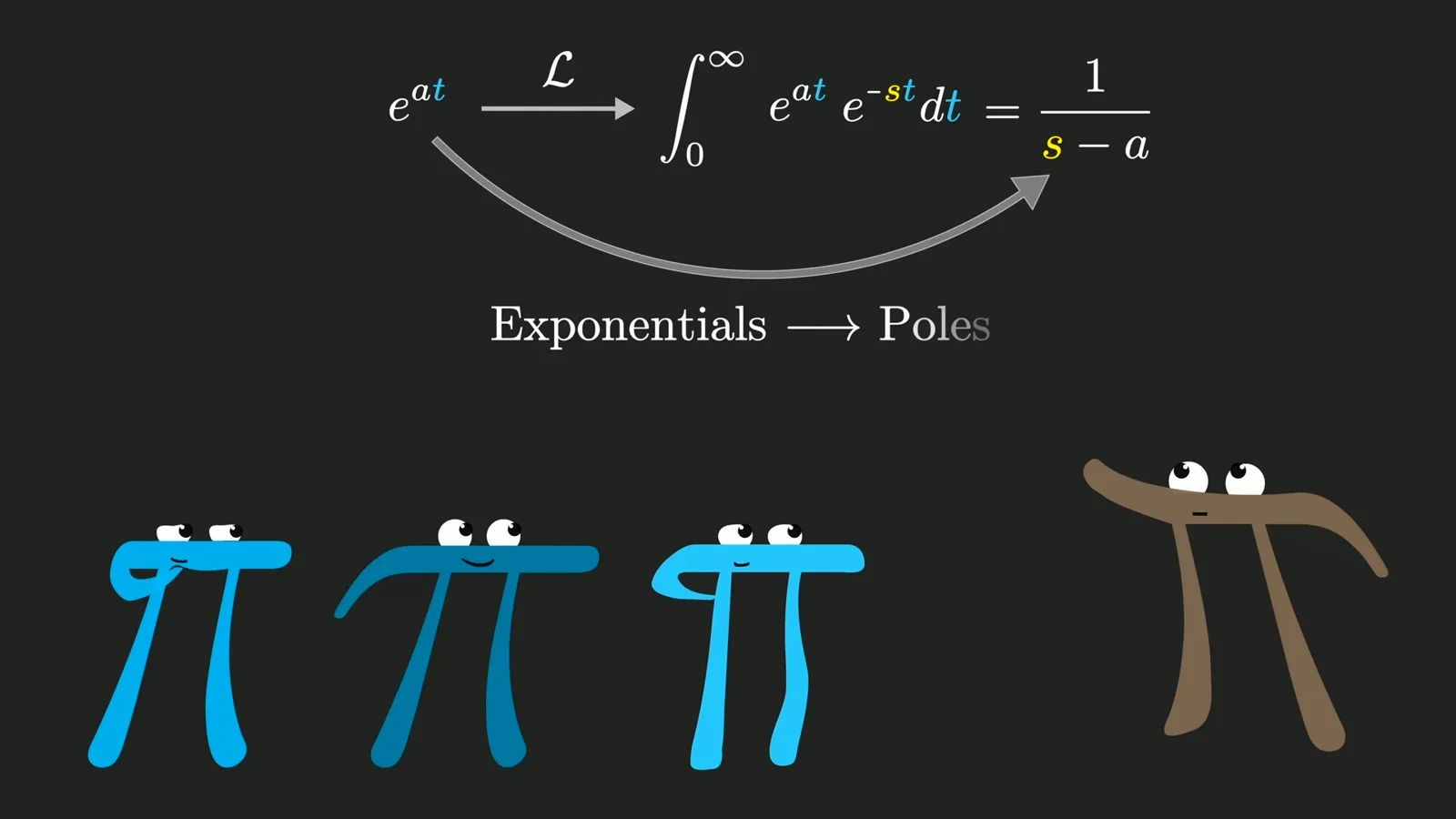
Nothing depends on the choice 1.5. In general, ℒ{e^(at)} = 1/(s−a) for Re(s) > Re(a), and its analytic continuation has a simple pole at s = a. That is the central connection between exponentials in time and poles in the s-plane.
Return to cosine. Linearity lets us transform its two half-weighted exponentials separately: ℒ{cos(t)} = ½/(s−i) + ½/(s+i), in the region where the integral converges. The resulting plot has two poles, one at i and the other at −i.
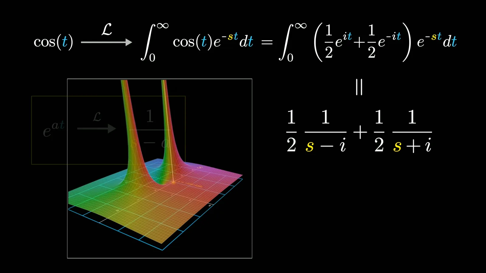
The visualization of the cosine integral is more intricate. For a small imaginary s, the rotating exponential multiplied by cosine traces a petal-like path. Unit-interval averages make a star-like vector sum. On the imaginary axis the ordinary sum need not converge; the plotted extension represents analytic continuation.
As the imaginary part of s approaches the cosine frequency, the components align more strongly and the accumulated integral grows. Near s = i, reducing the positive real part means less decay, so the value grows toward the pole.
Fourier and the wider picture
The cosine result connects with the Fourier transform and partial fractions. A later chapter will address more general functions and inversion.
This resembles the Fourier transform: on the imaginary axis the exponential probes oscillation frequencies. The conventions differ, including the lower integration limit of zero here rather than negative infinity, and convergence must be handled carefully. The Laplace transform also probes exponentials with growth or decay.
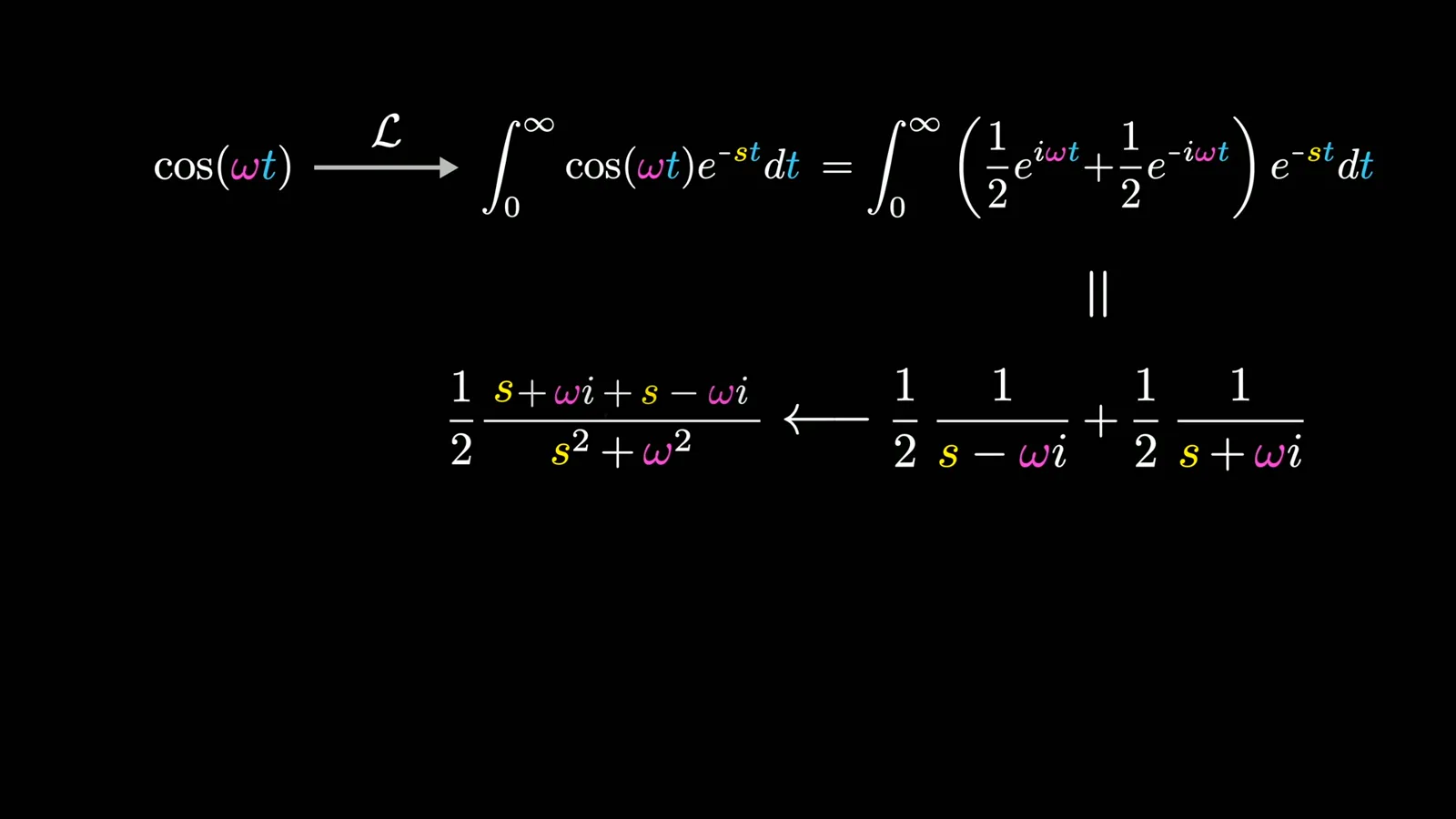
For cos(ωt), replace i with iω in the two fractions. Combining them gives the familiar table entry s/(s² + ω²). Conversely, direct integration followed by partial fraction decomposition recovers the poles ±iω and their coefficients of one half.
That reverse direction resembles practical use: calculate a transform and read its exponential pieces from the result. The worked differential-equation example moves to the next chapter. More generally, many functions require a continuous range of exponentials rather than a discrete sum; later lessons will develop inversion and its relationship to Fourier analysis.
Sur la même chaîne
 40:44EN
 3Blue1Brown· 16 oct. 2026Grant Sanderson: There's never been a better time to go into mathGrant Sanderson, Constantin Kogler · 3Blue1BrownStudents fear AI has solved mathematics. Grant Sanderson argues the opposite: even if machines prove theorems better than we do, the institution of math stays valuable—and this is a rare moment when newcomers can reshape it.
 51:55EN3Blue1Brown· 18 sept. 2026The last IMO problem AI could not solveGrant Sanderson · 3Blue1BrownGrant Sanderson walks through IMO 2025 Problem 6 — a tiling puzzle that frontier models missed — and the visual patience it takes to prove a construction is optimal.
 0:55EN3Blue1Brown· 24 juil. 2026The 64 Sugar Cubes Puzzle: Six Equal DistancesA 4×4×4 block has three colors; prove that six same-colored pairs share a distance.
 2:25EN3Blue1Brown· 12 juin 2026How Shannon Measured the Entropy of EnglishA guessing game helped Claude Shannon estimate how much information English text contains, and why prediction is central to compression.
 1:02EN3Blue1Brown· 10 juin 2026A Robot Walk and the Puzzle of Optimal Binary EncodingHow few bits does it take to send directions that occur with unequal frequencies?
 32:19EN3Blue1Brown· 7 juin 2026Reinventing Entropy: Why Prediction Helps Compress LanguageA robot’s movement code leads from prefix-free encoding to Shannon information and the entropy of language.