En 30 segundos
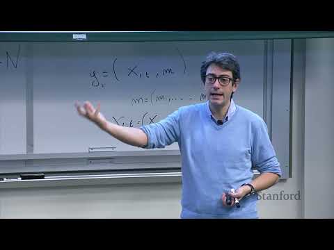
Sequential decisions can be solved by working backward: an optimal plan’s remaining actions must also be optimal for the remaining problem. In this 2019 Stanford lecture, Marco Pavone uses that principle to build dynamic programming, then adds random disturbances and state-dependent policies. A small inventory example illustrates the Bellman recursion. He closes with the computational and modeling limits that motivate approximate methods and reinforcement learning.
- 1An optimal plan has an optimal tailPavone proves by contradiction that a cheaper remaining path would also produce a cheaper complete path when costs are additive.
- 2Work backward to reuse the cost of future decisionsA small route example shows how dynamic programming avoids enumerating every complete path.
- 3Random disturbances change the solution from a sequence to a policyThe stochastic model optimizes expected cost and chooses an action as a function of the current state.
- 4An inventory example makes the Bellman recursion concreteThe lecture uses limited storage, uncertain demand and an ordering cost to calculate a final-stage action.
- 5Exact dynamic programming encounters several computational limitsPavone discusses dimensionality, unknown models and limited time, and introduces approximations in value and policy space.
Conclusiones
- Use the principle of optimality to reuse solutions to future subproblems when costs have the required additive structure.
- Under uncertainty, optimize a policy that maps observed states to actions rather than committing to one open-loop sequence.
- The Bellman recursion balances immediate cost against expected future cost.
- Exact dynamic programming faces state-space, modeling and time constraints; approximate value functions and policies are two alternatives.
Lee el texto editado por capítulos
Model sequential decisions and additive costs
Pavone starts with deterministic dynamics, control constraints and a finite-horizon cost, contrasting open-loop sequences with feedback.
Marco Pavone introduces high-level robot decisions such as whether to cross an intersection or change lanes. These choices must account for uncertainty in perception, the reconstructed environment and predictions of what other people will do.
The lecture develops a mathematical model for sequential decisions under uncertainty and a baseline solution method. Pavone frames reinforcement learning, the next topic in the course, as a family of approximate approaches related to these decision problems.
He recommends work by Dimitri Bertsekas for connecting optimal control and reinforcement learning within a common framework, even though the subjects often use different terminology.
Pavone begins with a deterministic discrete-time system. A state and control at time k determine the next state; at each state only certain controls are feasible, such as those respecting a road’s speed limit.
The finite-horizon objective adds a terminal cost to stage costs incurred at each time step. The initial problem chooses a sequence of controls to minimize the total cost from a given starting state.
A student identifies this as open-loop control: once the sequence is selected, the control at a given time does not depend on the state actually reached. A disturbance or model mismatch can therefore make a planned action inappropriate.
Pavone gives the example of a vehicle that has traveled farther than expected into a lower-speed zone. An open-loop plan might still command the previously scheduled higher speed because it does not respond to the observed state.
The discrete-time setting suits the high-level actions under discussion. The additive cost structure is especially important: it allows the total objective to be split into immediate and remaining costs.
Directly enumerating all possible control sequences can lead to a combinatorial explosion, especially with nonlinear constraints or nonconvex costs. The question is how to exploit structure to avoid solving every full sequence from scratch.
The principle of optimality
A contradiction argument shows why the tail of an optimal trajectory is optimal for its remaining subproblem.
The principle of optimality supplies that structure. Suppose an optimal path goes from A through B to E: its tail from B to E must itself be optimal for the subproblem starting at B.
Pavone proves the claim by contradiction. If a different route from B to E had lower cost, combining it with the original A-to-B segment would yield a cheaper A-to-E route.
Because costs are additive, the alternative tail would contradict the assumption that the original complete route is optimal. The point is not that an optimal solution is unique, but that an optimal path’s tail cannot be more costly than another feasible tail.
In the discrete-time formulation, applying the optimal control sequence from a known initial state generates an optimal state trajectory. Starting at a state reached along that trajectory, the remaining optimal controls solve the remaining finite-horizon problem.
Asked about the beginning versus the tail of a trajectory, Pavone says the stochastic case requires care: the backward, tail-subproblem perspective remains central. Under uncertainty, the formulation will use expectations and policies rather than a fixed sequence.
Suppose the optimal costs from C, D and E to a destination are already known. From B, the decision can compare the immediate cost of reaching each successor plus that successor’s known cost-to-go, instead of recomputing every tail.
Solve future subproblems backward
A route example and the Bellman recursion show how to reuse optimal costs instead of enumerating every path.
Pavone illustrates the method with a directed network of road segments. Starting at the destination, the cost to remain there is zero; he works backward, combining each edge cost with the already computed best cost from its endpoint.
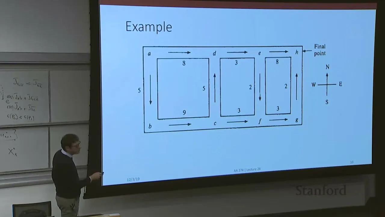
At a node with only one available action, the calculation is simply that edge cost plus the successor’s cost-to-go. At a node with several actions, compare the alternatives and retain the minimum.
A student catches an arithmetic slip in the example. Pavone corrects it and continues, emphasizing that the backward values can then be used to reconstruct the optimal path forward from the starting point.
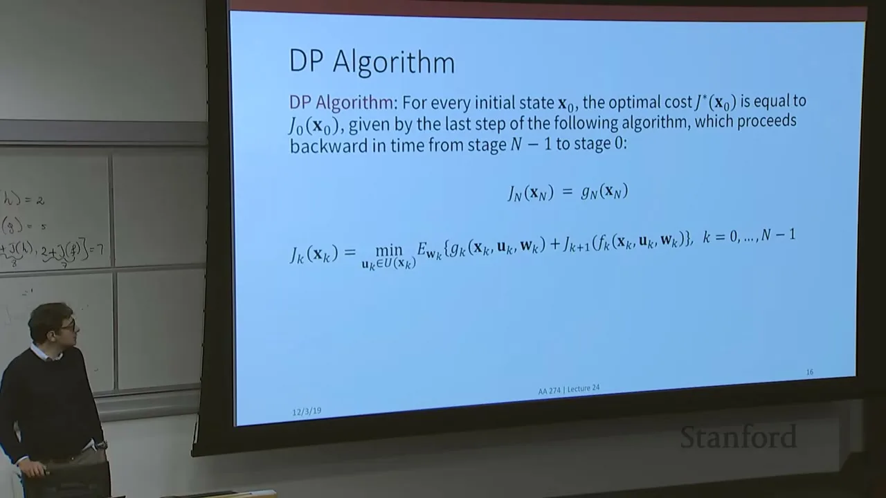
The formal dynamic-programming algorithm begins with the terminal cost. For each preceding time and each possible state, minimize the immediate cost plus the optimal cost-to-go at the next state.
Pavone interprets the recursion as balancing immediate gains or costs with future consequences. Although the computation proceeds backward, the resulting actions are executed forward in time.
A student asks about a partially observed state. Pavone says the same broad approach can be formulated over a belief distribution rather than a known state, but solving the recursion becomes much more difficult.
The model is discrete in time; a continuous-time problem can be discretized, while continuous-time dynamic programming has its own formulation. Many or continuously valued states also require approximation, quantization or interpolation.
If the exact algorithm can be run to completion under its assumptions, it yields a global optimum for the modeled problem. Control constraints can reduce the number of candidate actions that must be checked.
Asked about non-additive costs, Pavone notes that some trajectory-wide probabilities or risk measures couple stages. Such objectives may need reformulation or approximation before the simple recursion applies.
Add uncertainty and state-dependent policies
Random disturbances and a Markov assumption lead to an expected-cost formulation and a stochastic Bellman recursion.
For the stochastic case, the state transition also depends on a random disturbance. Its probability distribution may depend on the current state and action, but the Markov assumption rules out additional dependence on earlier history once those are given.
Under uncertainty, Pavone seeks a closed-loop policy: a function mapping each possible state to an action. A fixed open-loop sequence cannot respond to the different states produced by random disturbances.
Stage and terminal costs can be random, so this formulation ranks policies by expected total cost. It is risk-neutral: it optimizes the average rather than directly controlling variance or a worst-case quantile.
The Markov property and additive objective permit a stochastic version of the principle of optimality. The tail policy remains optimal for the remaining problem from a reached state, with probabilities included in the reasoning.
The Bellman recursion still moves backward from terminal cost. The additional operation is an expectation over the current disturbance when comparing immediate cost plus the next state’s cost-to-go.
Inventory control and the limits of exact methods
A small warehouse example illustrates the calculation; dimensionality, modeling and time motivate approximate methods.
Pavone introduces a small inventory problem. The state is current stock, the action is how much to order, and random demand determines the next stock level, which cannot drop below zero.
The warehouse holds at most two units after ordering. Demand is zero with probability 0.1, one unit with probability 0.7 and two units with probability 0.2; the example combines ordering cost with a quadratic term and uses a three-step horizon.
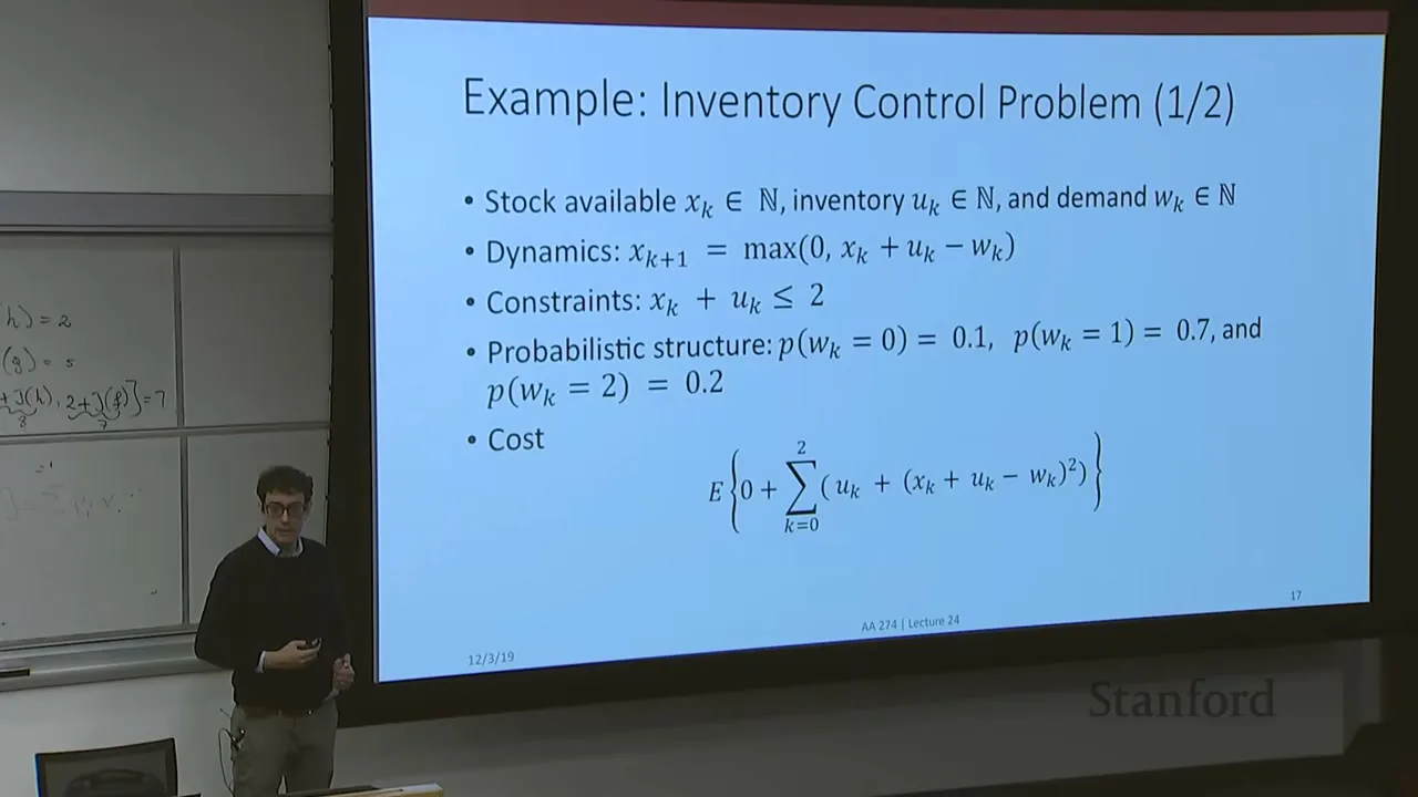
The terminal cost is set to zero. Dynamic programming starts there, then computes the optimal cost-to-go for each possible stock level at the previous time before moving backward again.
For the illustrated final decision with zero stock, the feasible orders are zero, one or two units. Pavone evaluates expected cost over the three demand outcomes and obtains order one, with an optimal cost-to-go of 1.3 for that state.
The example shows how to construct a policy for each state and time, but exact dynamic programming still suffers from a curse of dimensionality: the number of state combinations grows rapidly with the number of state variables.
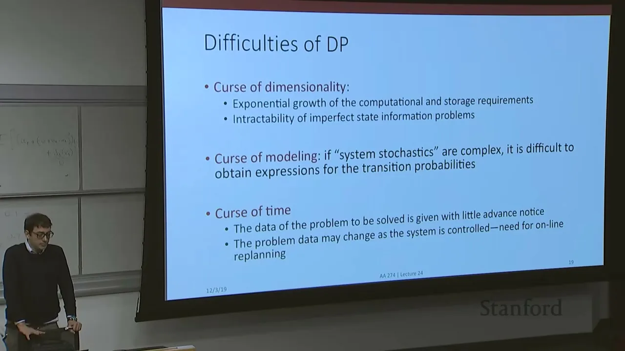
Partial observability can make the state of the optimization a belief distribution, further increasing computational difficulty. Another limitation is modeling: transition probabilities, such as a person’s response to a robot, may be unknown and need to be learned.
Time is a third constraint. Data or system conditions may change while the controller is operating, leaving too little time to recompute a complete exact policy.
Approximate dynamic programming addresses these limits. One approach approximates the optimal cost-to-go with a surrogate, for example by solving a simpler problem, using an approximate optimizer, learning a function such as a neural network, or aggregating states.
A second approach restricts the policy to a parameterized family and optimizes the parameters rather than searching over all possible functions. Pavone says the next lecture will explore such approximate and learning-based approaches.
Más de este canal
 1:04:32EN
 Stanford Online· 6 nov 2026How particle filter SLAM separates a robot’s path from its mapMarco Pavone · Stanford UniversityMarco Pavone derives the conditional independence that makes a particle-based mapping algorithm practical.
 1:47:01ENStanford Online· 5 nov 2026How LLM systems fit large models into hardware and serve them fasterAfshine Amidi, Shervine Amidi · Stanford UniversityAfshine and Shervine Amidi explain FlashAttention, distributed training and inference optimizations from memory movement to speculative decoding.