In 30 seconds
In a lecture at UC Santa Cruz, the 3Blue1Brown narrator builds the volume formula for an n-dimensional ball from probability, Archimedes’ projection and a two-dimensional recurrence. He then explains the gamma function, shrinking unit-ball volumes and the concentration of volume near the boundary.
- 1Probability becomes geometryRandom coordinates form a point in a cube; the squared-sum condition picks out the ball inside it.
- 2A surprising packing puzzleThe central ball tangent to unit balls at cube corners has radius √n − 1 and protrudes beyond a certain bounding cube in ten dimensions.
- 3Archimedes in more dimensionsA volume-preserving projection relates a higher-dimensional sphere’s boundary to a lower-dimensional ball times a circle.
- 4The recurrenceUnit-ball volumes satisfy cₙ = (2π/n)cₙ₋₂.
- 5Near the boundaryIn n dimensions, shrinking the radius to 99% retains only 0.99ⁿ of the volume.
Takeaways
- The probability that n independent uniform numbers in [−1, 1] have squared sum at most one is the unit n-ball volume divided by 2ⁿ.
- The radius-r n-ball has volume π^(n/2)rⁿ/Γ(n/2 + 1).
- A two-dimension recurrence multiplies the unit-ball volume by 2π/n.
- Among integer dimensions, the numerical unit-ball volume is largest in dimension five and tends to zero as dimension grows.
- A fixed fractional shell near the boundary contains nearly all the volume in sufficiently high dimensions.
Read the edited text by chapter
A probability question
Random coordinates turn an analytical probability problem into a question about ball and cube volumes.
The 3Blue1Brown narrator introduces a formula he considers underappreciated: the volume of a ball in any number of dimensions. He wants the audience to understand both its meaning and its derivation.
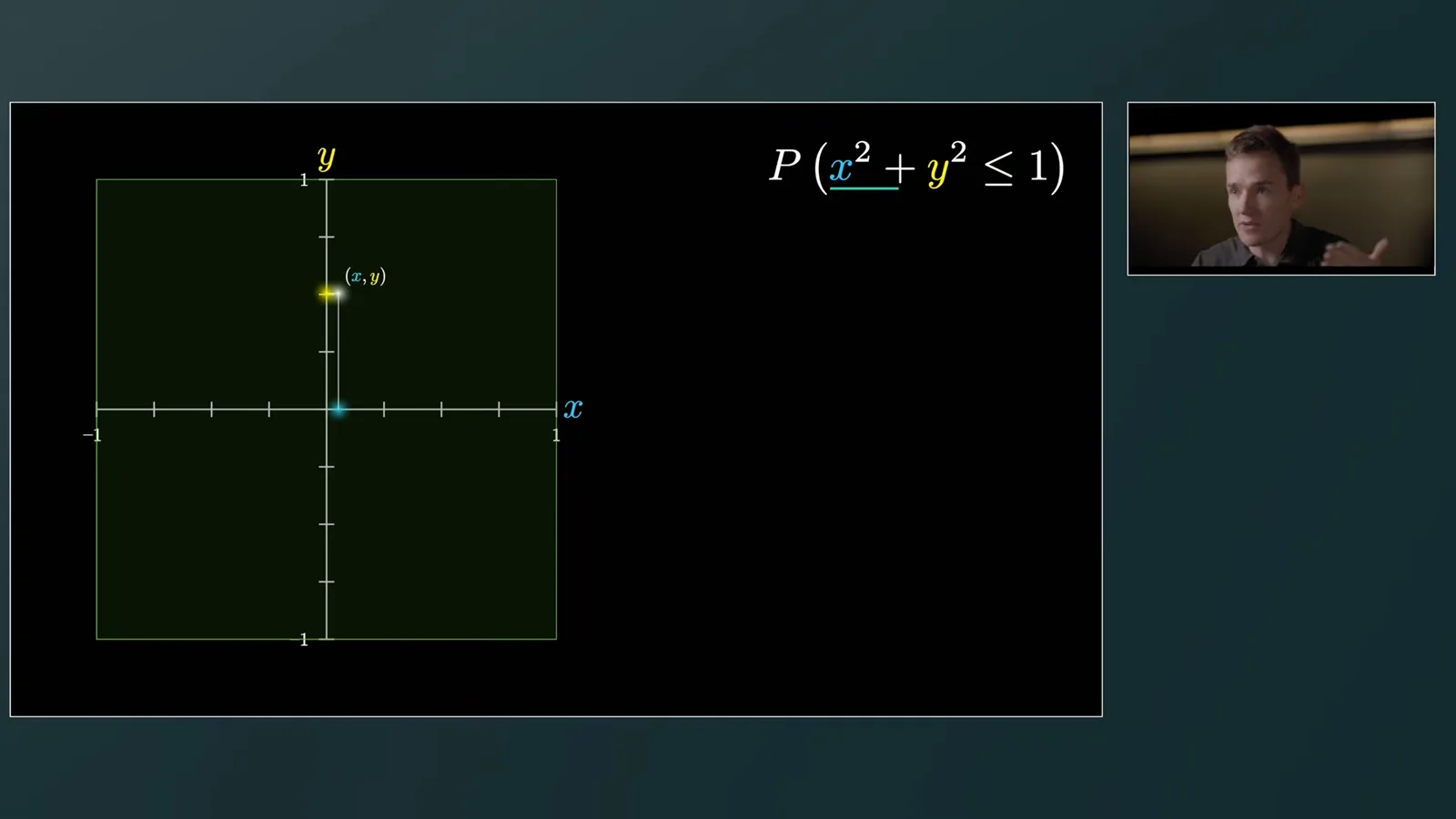
For the first puzzle, choose independent uniform random numbers x and y between −1 and 1. What is the probability that x² + y² is at most 1?
The pair (x, y) is a uniformly chosen point in a 2-by-2 square. The inequality describes the unit disk, so the probability is its area divided by the square’s area: π/4.
With three independent coordinates the same argument uses a unit ball inside a cube of side 2. Its volume is 4π/3, and the probability is (4π/3)/8 = π/6.
Nothing prevents the question from having four or a hundred coordinates. The answer becomes the volume of the corresponding unit ball divided by the volume 2ⁿ of the n-dimensional cube.
A high-dimensional point can simply represent a long list of numbers. The narrator notes that machine-learning representations offer a familiar setting where geometric language can help reason about such lists.
The corner-ball puzzle
A simple construction shows how intuition from two and three dimensions can mislead in higher dimensions.
A second puzzle warns against relying too heavily on low-dimensional pictures. Put unit circles at the four corners of a square whose corners are (±1, ±1), then grow a central circle until it touches them.
The origin is √2 from each corner, so the central circle’s radius is √2 − 1. In three dimensions the corresponding distance is √3, giving a central radius of √3 − 1.
Repeated applications of the ordinary Pythagorean theorem give the distance to an n-dimensional corner as √n. With a unit ball at each corner, the central tangent ball therefore has radius √n − 1.
In four dimensions this radius is 1. In ten dimensions it is approximately 2.16, so the central ball extends beyond the faces of the larger side-4 cube that contains the corner balls.
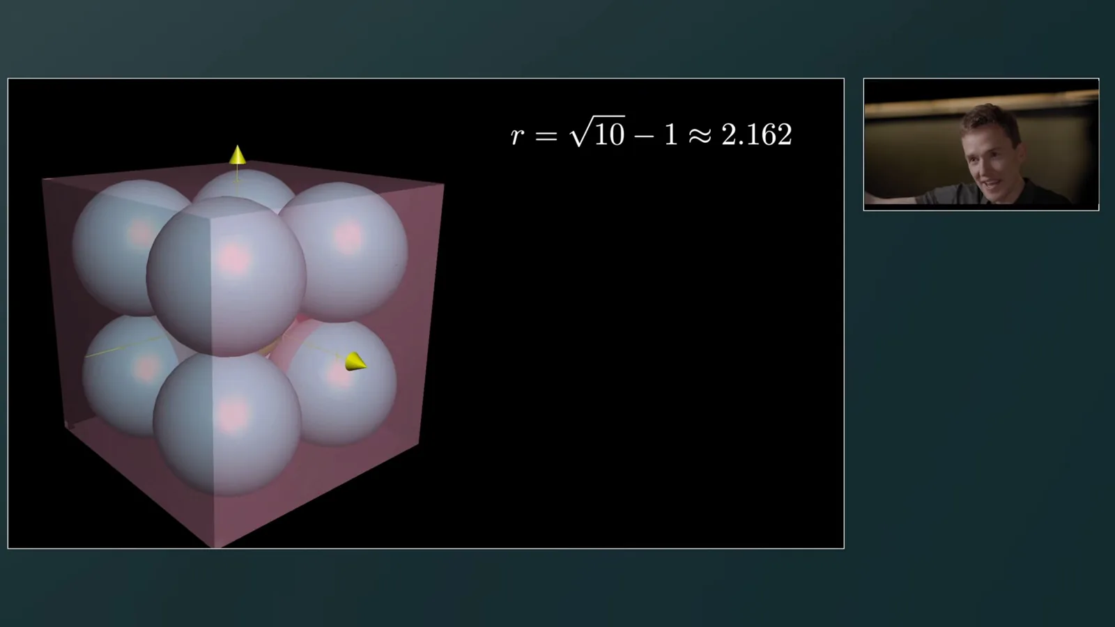
The narrator rejects the description that high-dimensional spheres are “spiky”: a sphere still consists of points at a fixed distance from its center. The surprising geometry comes from the distance between a high-dimensional cube’s center and its many corners.
A cube face remains a fixed distance from the center while the corner distance grows as √n. A distorted low-dimensional sketch can suggest the effect, but it cannot faithfully depict all 2ⁿ corners.
Building a volume table
The lecture relates boundary measure to the derivative of ball volume and revisits the one-dimensional case.
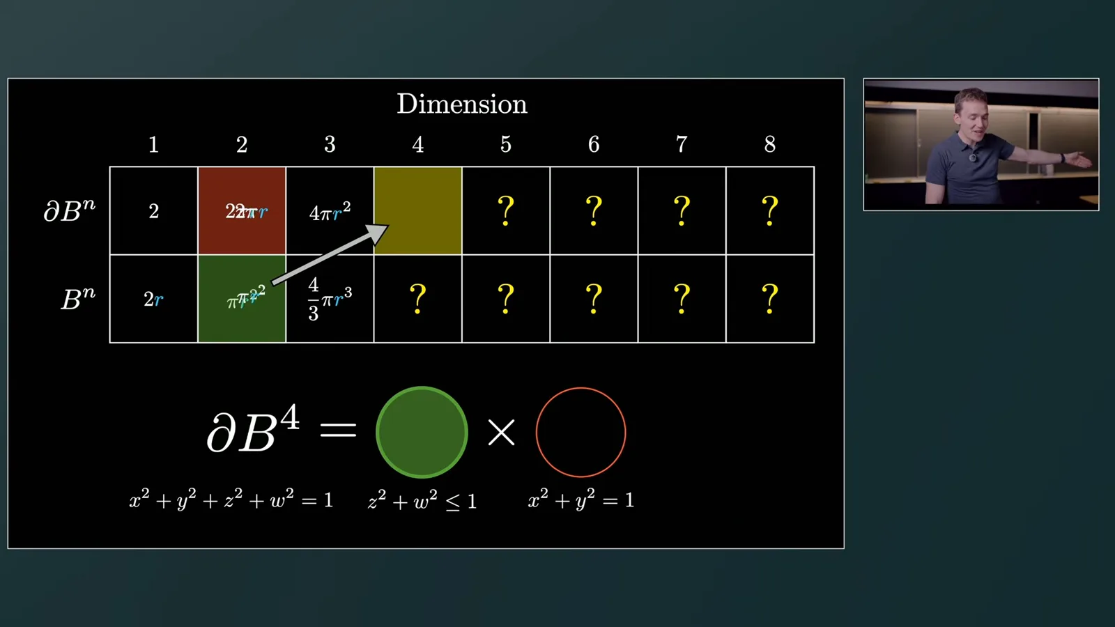
To derive the volume formula, the narrator makes a table of ball volumes and boundary measures in different dimensions. Familiar entries include circle area πr², circumference 2πr, sphere surface area 4πr² and ball volume 4πr³/3.
The boundary measure is the derivative of ball volume with respect to radius. A small increase dr adds a thin shell, whose volume is approximately boundary measure times dr; the approximation becomes exact in the derivative limit.
Going in the other direction, integrate boundary measures over radius. For instance, integrating a quantity proportional to r² produces an r³ term divided by 3.
A one-dimensional ball of radius r is the interval from −r to r, with length 2r. Its boundary consists of two points; counting them gives boundary measure 2, matching the derivative.
Archimedes and higher dimensions
An area-preserving projection suggests a two-dimensional step in the volume table. Integrating gives the next ball volume.
For a sphere in three dimensions, Archimedes projected small surface patches onto the enclosing cylinder. One direction stretches while another contracts, and the local area factors cancel.
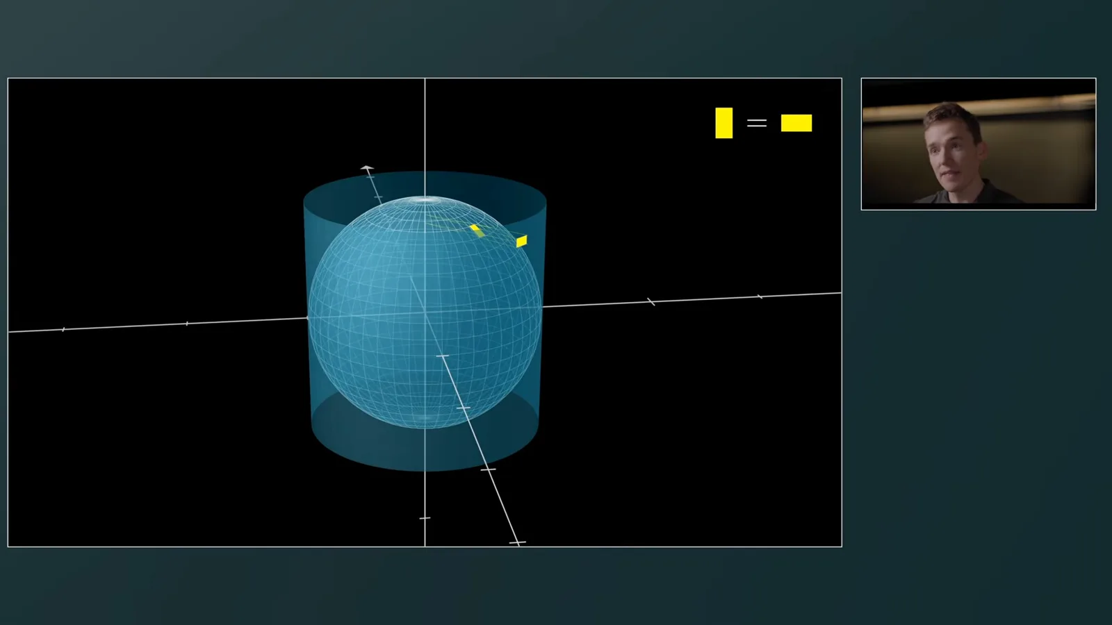
In the illustration, the stretch around the axis is R/d, where R is the sphere radius and d is the distance to the axis. The perpendicular contraction is d/R, so their product is one.
The cylinder can be unwrapped into a rectangle of width 2πr and height 2r. Its area, 4πr², is therefore also the sphere’s surface area.
The narrator recasts this as a step in the volume table: the sphere boundary’s measure is the length of a one-dimensional ball times the circumference of a two-dimensional ball. He calls the movement through the table a knight’s move.
For a point on the three-dimensional sphere, first choose z in [−r, r]; the remaining x and y lie on a circle. Its radius changes with z, so multiplying by a fixed circumference is not automatic; the projection is what justifies the area calculation.
In four dimensions, first choose two coordinates inside a disk. The remaining two lie on a circle whose radius depends on that choice, but the generalized projection again balances stretching and compression for the boundary measure.
The resulting boundary measure of the four-dimensional ball is 2π²r³. Integrating with respect to r gives volume π²r⁴/2. The product description concerns measure after projection, not literal equality of the shapes.
A numerical simulation can check the result empirically: sample four coordinates uniformly from [−1, 1] and count how often their squared sum is at most one. It approaches the four-ball volume divided by 2⁴, although simulation is not a proof.
The same construction extends to higher dimensions by separating two coordinates for a circle and the others for a lower-dimensional ball. The two-dimensional choice is what gives the canceling stretch and compression.
Each step multiplies by 2πr for the boundary and then integrates. If cₙ is the volume of the unit n-ball, this yields the recurrence cₙ = (2π/n)cₙ₋₂.
The formula and half factorials
The recurrence leads to a unified formula involving a generalized factorial and the gamma function.
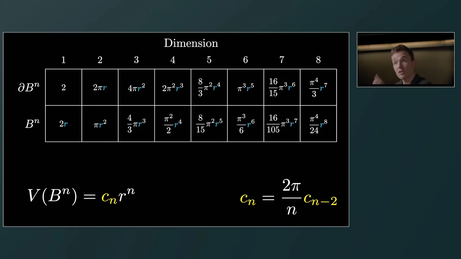
The recurrence allows a volume in eight dimensions to be reduced to six, four, two and finally zero dimensions. Taking the zero-dimensional unit ball to have volume 1 provides the even-dimensional base case.
Following the even-dimensional recurrence produces powers of π in the numerator and a factorial in the denominator. Including radius gives Vₙ(r) = π^(n/2)rⁿ/(n/2)! when n is even.
The same recurrence also works in odd dimensions, but the notation then asks for half-integer factorials. The one-dimensional case requires (1/2)! = √π/2; further half-integer values follow recursively.
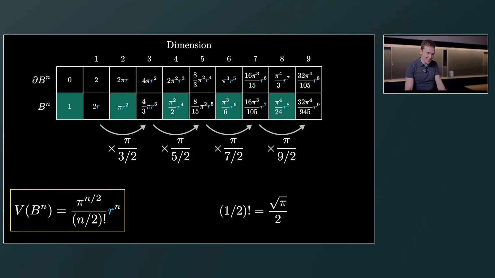
The gamma function provides a standard extension of factorials: x! = Γ(x + 1). Thus the unified formula is Vₙ(r) = π^(n/2)rⁿ/Γ(n/2 + 1), for integer n ≥ 0.
The narrator notes another route through Gaussian integrals and the gamma function. That separate line of reasoning agrees with the half-factorial values suggested by the volume recurrence.
Why unit-ball volumes shrink
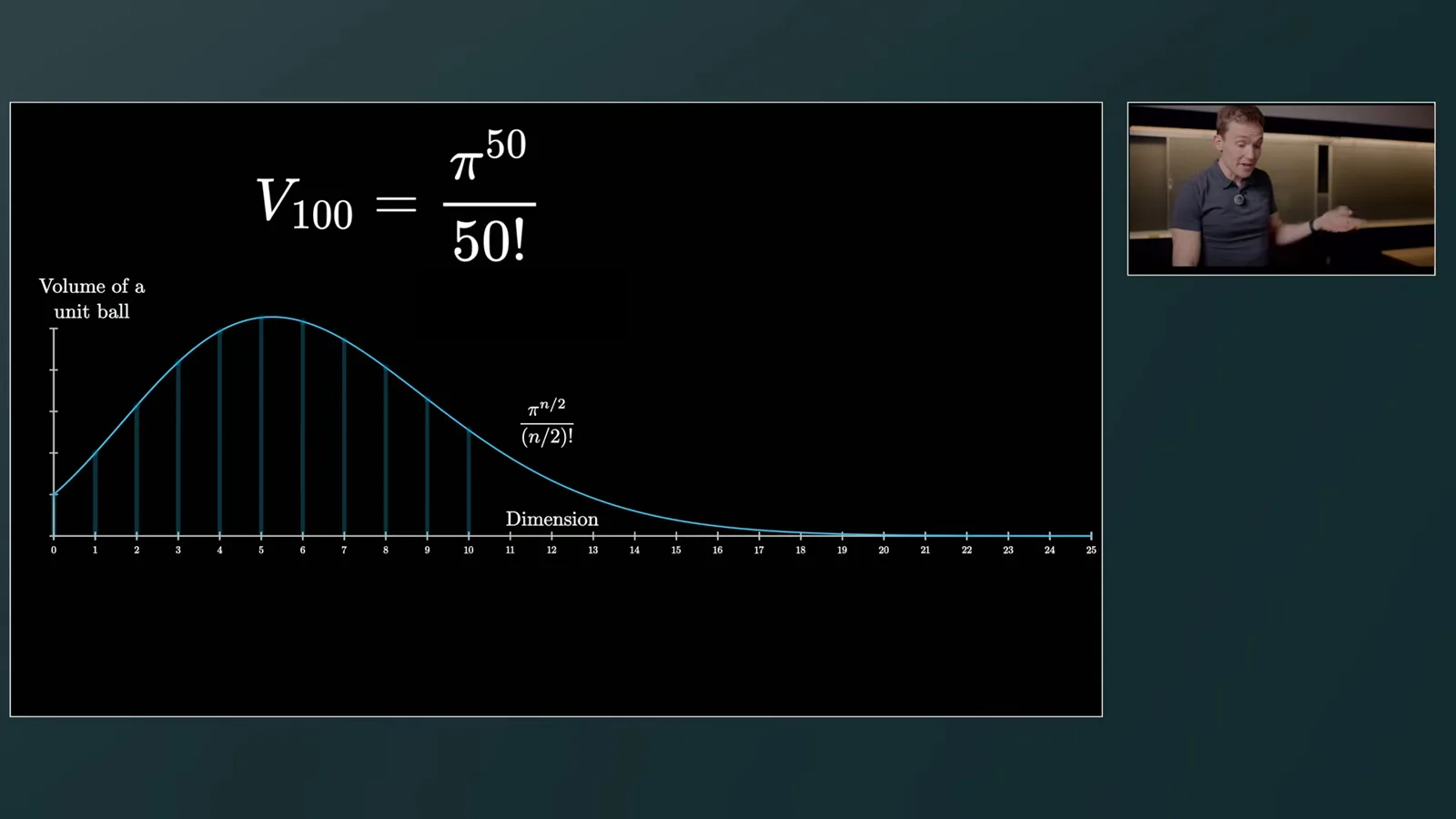
Numerical unit-ball volumes peak at dimension five, then approach zero. The comparison uses consistent unit conventions.
For unit radius, the numerical volumes rise from 1 in dimension zero to 2, π and 4π/3 in the next dimensions. They continue increasing through dimension five, then decrease for the positive integer dimensions that follow.
The recurrence explains the turning point: each two-dimensional jump multiplies by 2π/n. Once n grows beyond 2π, that multiplier is less than one, and subsequent steps in each parity sequence shrink.
In 100 dimensions, the unit-ball volume is π⁵⁰/50!, approximately 2.37 × 10⁻⁴⁰ in the chosen units. The probability from the opening puzzle is smaller still because it divides this volume by 2¹⁰⁰.
Where the volume lies
A fixed fractional shell contains almost all volume in high dimensions. The lecture finishes by interpreting the formula without comparing incompatible units.
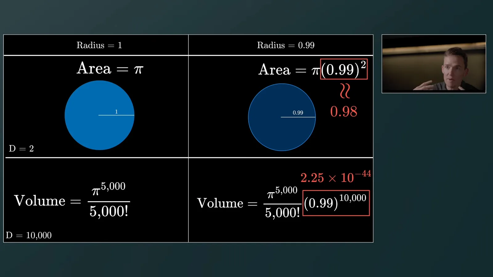
A separate phenomenon concerns where volume is located. For a unit disk, the portion within 1% of the boundary is 1 − 0.99², roughly 2% of the area.
In n dimensions, scaling the radius to 0.99 retains a fraction 0.99ⁿ of the volume. At n = 10,000 this is about 2.25 × 10⁻⁴⁴, so nearly all volume lies in the outer 1% shell.
The narrator also points to concentration near an equator of a high-dimensional sphere: cross-sections even slightly away from it shrink rapidly as the dimension grows.
Comparing a length, area and higher-dimensional volume directly mixes units. A dimensionless interpretation compares each unit ball with a unit-side cube in the same dimension; the formula is the ratio under that convention.
In the corner-ball construction, there are 2ⁿ unit balls and the larger cube has volume 2ⁿ. Their total-volume ratio therefore equals the unit n-ball volume, giving another way to interpret its smallness in high dimensions.
The lecture closes by connecting familiar formulas and factorials through a more general pattern. Their shared structure is easier to see once the problem is viewed across dimensions.
The opening animation
The narrator explains the projected higher-dimensional latitude animation shown at the start.
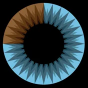
In a final note, the narrator explains the opening animation: it shows latitude spheres of a four-dimensional sphere projected into three dimensions, with the apparent shapes changing as the higher-dimensional perspective rotates.
More from this channel
 40:44EN
 3Blue1Brown· Oct 16, 2026Grant Sanderson: There's never been a better time to go into mathGrant Sanderson, Constantin Kogler · 3Blue1BrownStudents fear AI has solved mathematics. Grant Sanderson argues the opposite: even if machines prove theorems better than we do, the institution of math stays valuable—and this is a rare moment when newcomers can reshape it.
 51:55EN3Blue1Brown· Sep 18, 2026The last IMO problem AI could not solveGrant Sanderson · 3Blue1BrownGrant Sanderson walks through IMO 2025 Problem 6 — a tiling puzzle that frontier models missed — and the visual patience it takes to prove a construction is optimal.
 0:55EN3Blue1Brown· Jul 24, 2026The 64 Sugar Cubes Puzzle: Six Equal DistancesA 4×4×4 block has three colors; prove that six same-colored pairs share a distance.
 2:25EN3Blue1Brown· Jun 12, 2026How Shannon Measured the Entropy of EnglishA guessing game helped Claude Shannon estimate how much information English text contains, and why prediction is central to compression.
 1:02EN3Blue1Brown· Jun 10, 2026A Robot Walk and the Puzzle of Optimal Binary EncodingHow few bits does it take to send directions that occur with unequal frequencies?
 32:19EN3Blue1Brown· Jun 7, 2026Reinventing Entropy: Why Prediction Helps Compress LanguageA robot’s movement code leads from prefix-free encoding to Shannon information and the entropy of language.