Taylor Series: Turning Derivatives Into Approximations

When I first learned Taylor series, I did not appreciate how often they appear in mathematics, physics and engineering. Their power is to approximate a complicated function with a polynomial, which is often easier to calculate, differentiate or integrate.

A pendulum offers an example. Its height above the lowest point is proportional to 1 − cos θ. For small angles measured in radians, replacing cos θ with 1 − θ²/2 simplifies the expression and makes its relationship to other oscillations clearer.

The graphs of cos x and 1 − x²/2 lie close together near zero. How can we construct that quadratic rather than guess it? Start with P(x) = c₀ + c₁x + c₂x² and choose the three coefficients to match information about cosine at zero.

First match the value. Because cos 0 = 1 and P(0) = c₀, set c₀ = 1. Changing the other coefficients will not alter that value at zero, so they remain available to control the shape.

Next match the tangent slope. The derivative of cosine is −sin x, which is zero at x = 0. The derivative of P is c₁ + 2c₂x, so its slope at zero is c₁. Setting c₁ = 0 makes both curves flat there.

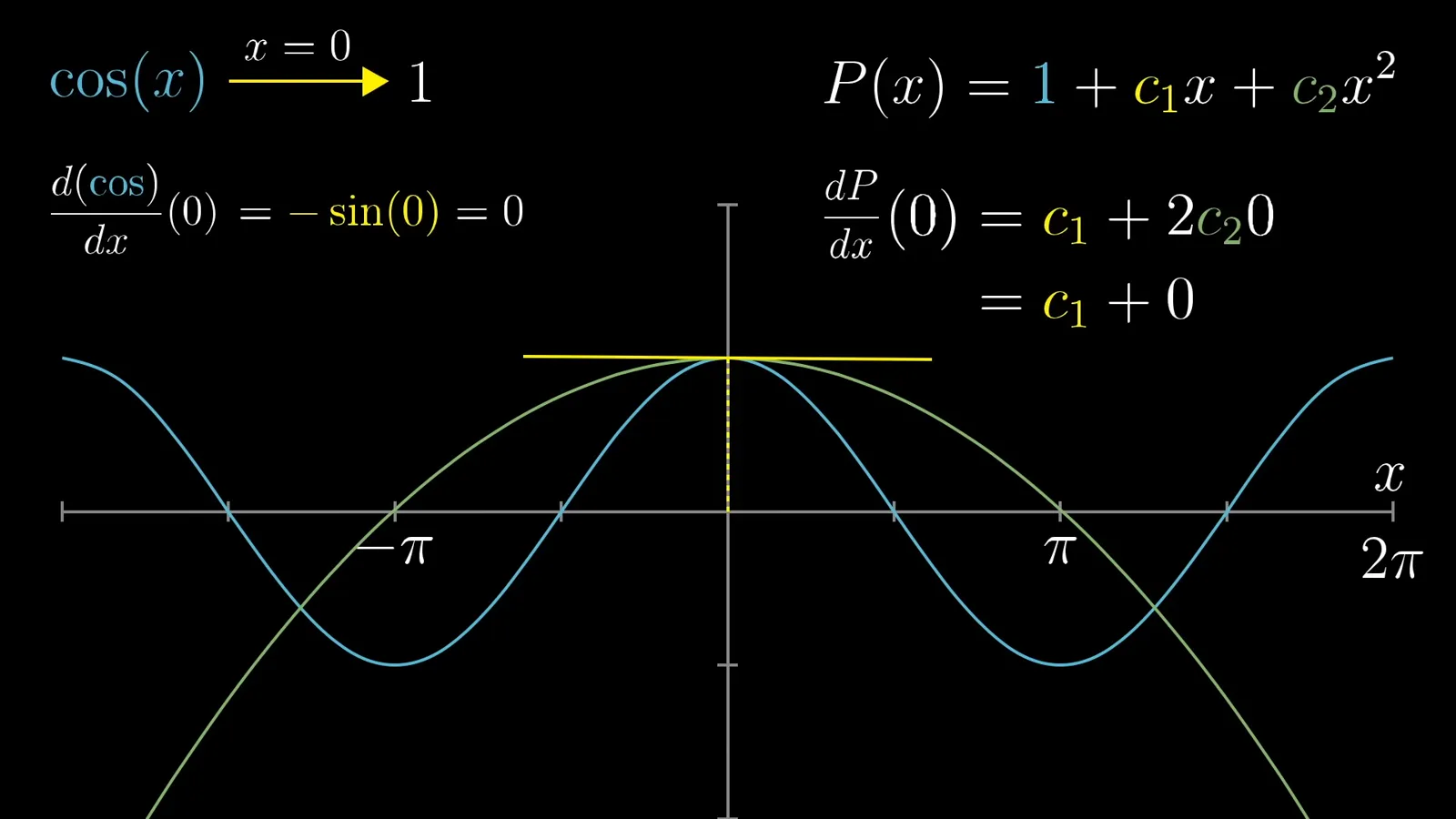
Finally match how the slope changes. The second derivative of cosine is −cos x, or −1 at zero. The second derivative of P is 2c₂, so c₂ = −1/2. The result is P(x) = 1 − x²/2.

At x = 0.1 radians, the polynomial gives 0.995, very close to cos(0.1). Each coefficient had a job: match the value, the first derivative, and the second derivative. This gives a local approximation, not a promise of equal accuracy far from zero.

We can add higher powers and match more derivatives. The third derivative of cosine is sin x, so it is zero at zero. A cubic term would have coefficient zero: the quadratic Taylor polynomial is also the cubic Taylor polynomial here.

The fourth derivative of cosine is cosine itself, giving 1 at zero. Differentiating c₄x⁴ four times gives 4!c₄ = 24c₄, so c₄ = 1/24. The improved polynomial is 1 − x²/2 + x⁴/24.

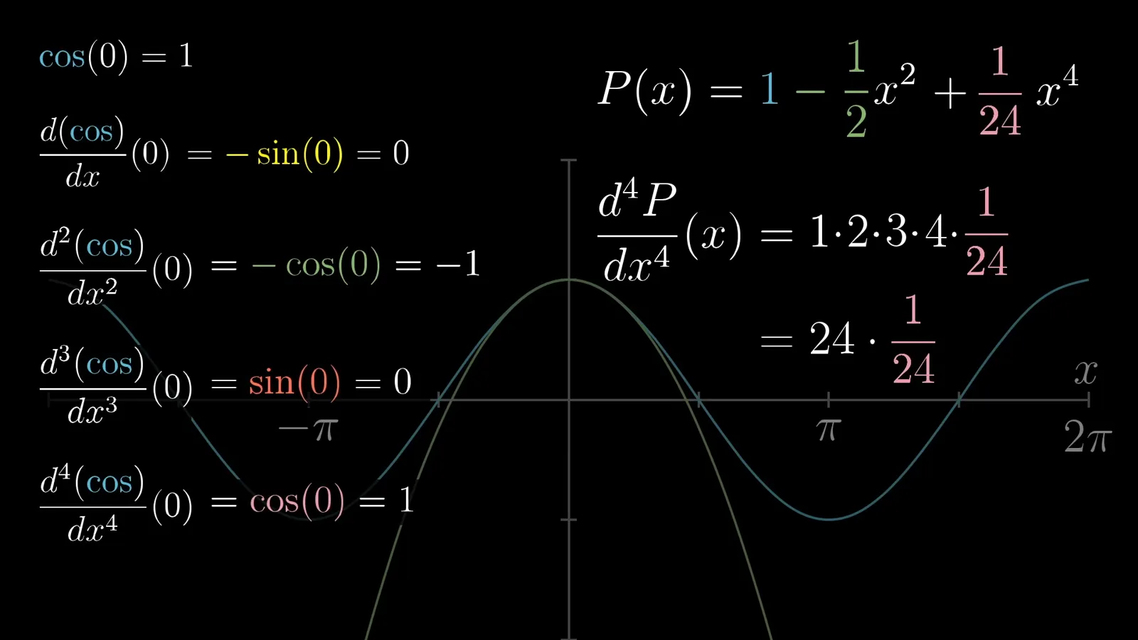
This explains the factorial. Repeatedly differentiating xⁿ brings down n, then n − 1, and so on, producing n!. To obtain the desired nth derivative at the center, divide that derivative’s value by n! when choosing the coefficient.

Higher-order terms do not disturb the derivatives already matched at zero: after fewer than n derivatives, an xⁿ term still contains a factor of x and vanishes at the center. Each new coefficient can therefore match another derivative without undoing earlier matches.

For an approximation centered at a different input a, use powers of x − a. At x = a, those powers vanish just as powers of x did at zero. The same construction now matches the function and its derivatives at a.

The cosine derivatives cycle through cos x, −sin x, −cos x and sin x. At zero their values cycle through 1, 0, −1, 0. Dividing each value by its factorial gives the coefficients of successive Taylor polynomials.

In general, the degree-n Taylor polynomial of f centered at a is the sum from k = 0 to n of f⁽ᵏ⁾(a)(x − a)ᵏ/k!. Its terms match the value and successive derivatives at a. More terms can improve a local approximation, although the resulting polynomial is more complex.

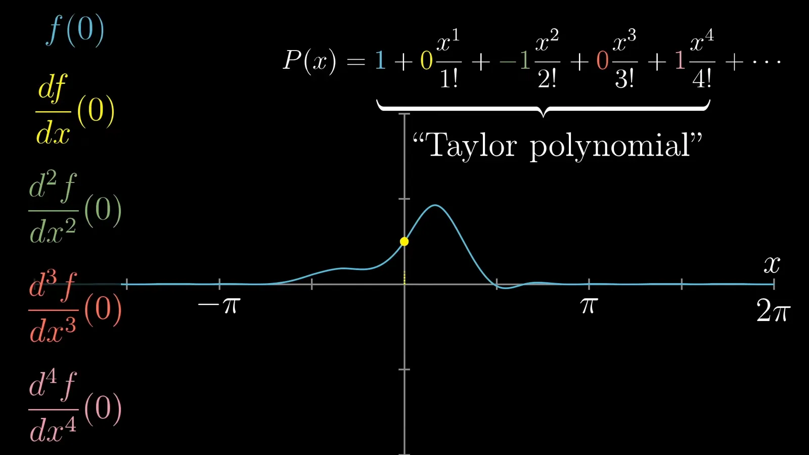
For eˣ centered at zero, every derivative is eˣ and every derivative at zero equals 1. Its Taylor polynomials therefore begin 1 + x + x²/2! + x³/3! + …, stopping at the desired degree.

There is also a geometric way to see the second-order term. Imagine a function measuring area under a curve up to a variable right endpoint. By the fundamental theorem of calculus, the height of the curve is the derivative of that area function.

Moving the endpoint from a to x adds approximately a rectangle of width x − a. To improve the estimate, include the small triangle caused by the changing height. Its base is x − a and its height is approximately f″(a)(x − a), where f is the area function.

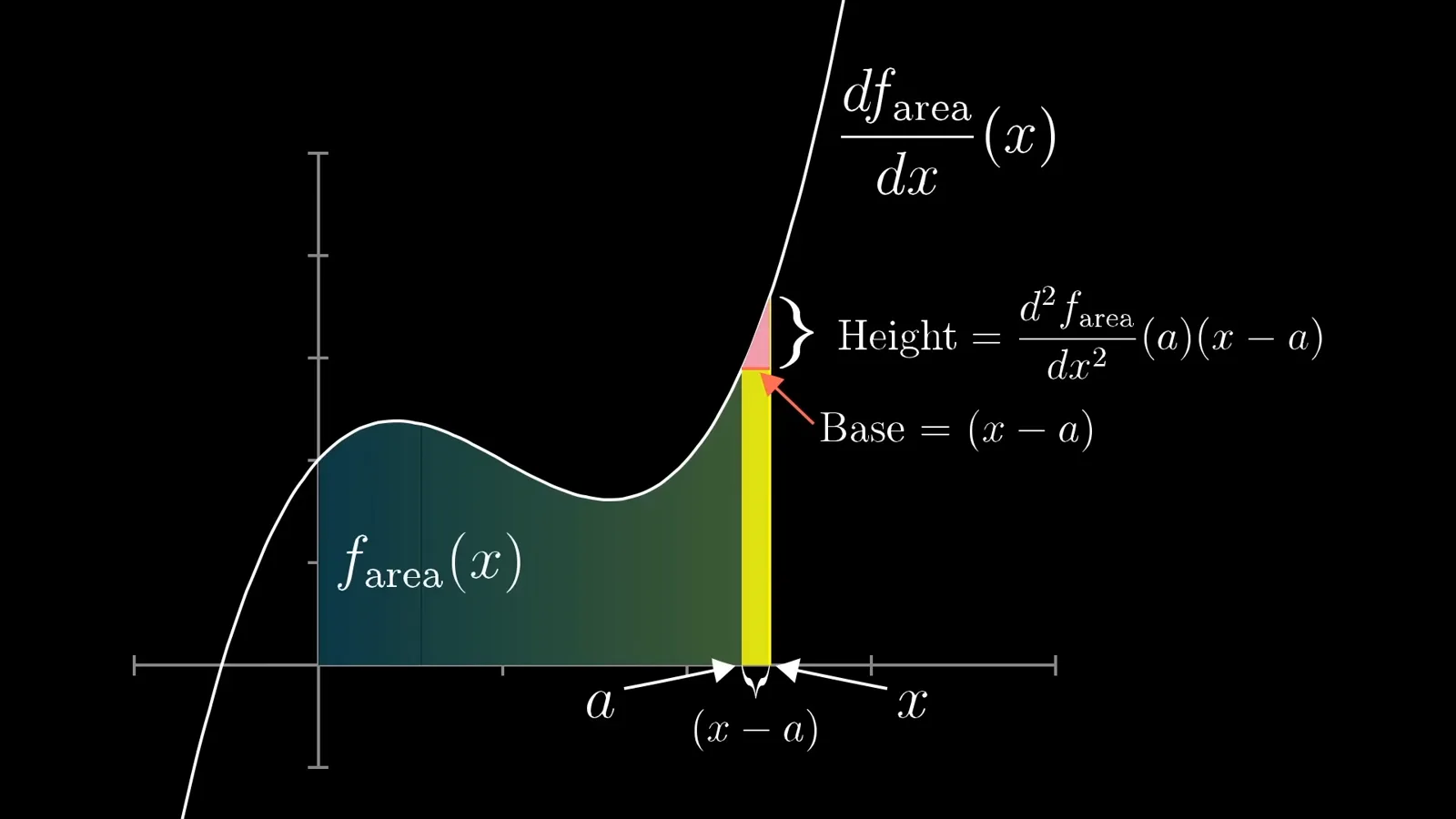
The triangle’s area is approximately ½f″(a)(x − a)². Adding the original area, the rectangle and the triangle gives the second-order Taylor approximation. The three terms have visible geometric meanings rather than being just symbols in a formula.

A Taylor polynomial stops after finitely many terms. A Taylor series considers the limit of the partial sums as the number of terms grows without bound. If those partial sums approach a particular value, the series converges to that value.

For eˣ centered at zero, adding more terms converges to eˣ for every real x. For example, at x = 1 the partial sums approach e. Local derivative information at one point determines the function throughout this particular domain.

Not every Taylor series behaves that way. The series for ln x centered at 1 converges to ln x for 0 < x < 2 and also at x = 2; it diverges at x = 0 and for x > 2. The endpoint x = 2 is conditional convergence, a detail beyond the video’s interval illustration.

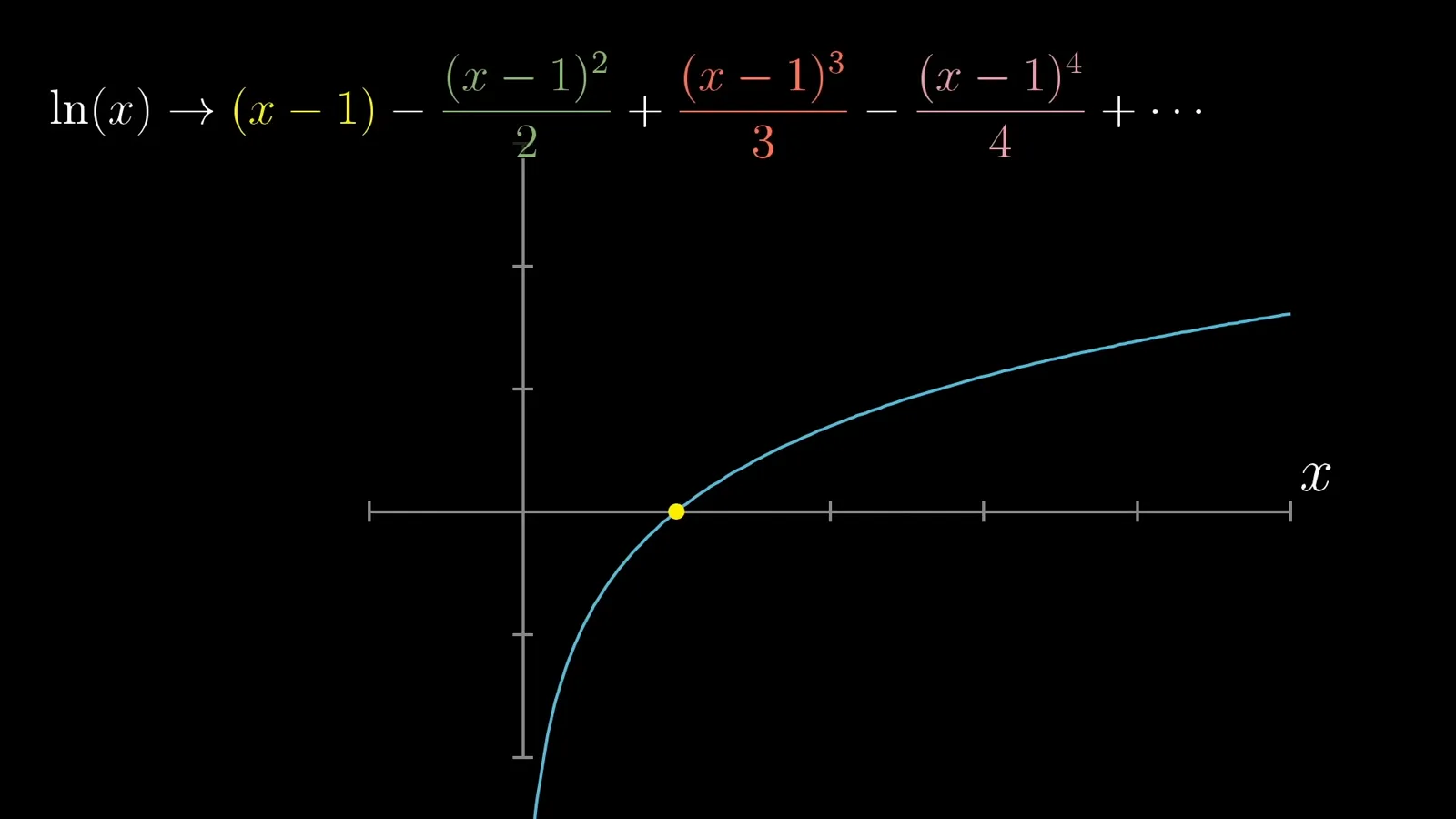
The radius of convergence describes the distance from the center within which a power series converges; boundary points need separate examination. More advanced work can bound approximation errors and test convergence, but the central intuition remains translating derivatives at one point into nearby approximations.