Vilas Winstein: Simulating Phase Changes with the Boltzmann Distribution

This lesson builds a simulation of a liquid–vapor phase transition. To understand it, we will derive the Boltzmann distribution, construct a sampling algorithm and explore the surprising behavior it produces. A second video on Spectral Collective takes up a simpler model that can be analyzed more completely.

Phase transitions are not chemical reactions: ice, liquid water and steam all contain H₂O. They differ in how molecules interact and in their large-scale behavior. Ice has a rigid structure, water can transmit ripples, and a small local disturbance in steam has little effect far away.

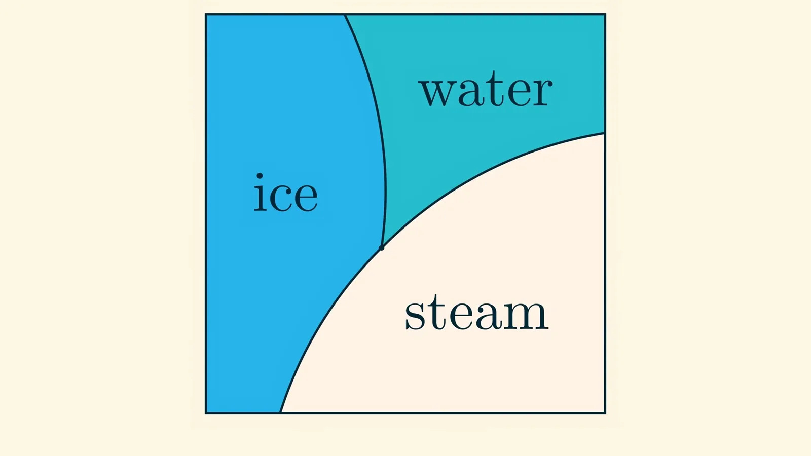
A phase diagram describes equilibrium behavior after a system has had time to settle at a given temperature and pressure. Crossing a phase boundary produces a discontinuity in equilibrium properties; it does not mean that boiling or freezing must happen instantaneously in real time.

At sufficiently high temperature and pressure, water can become a supercritical fluid. One can move continuously through that region from liquid-like to gas-like behavior without crossing a phase boundary. Our simplified model focuses on this part of the diagram.

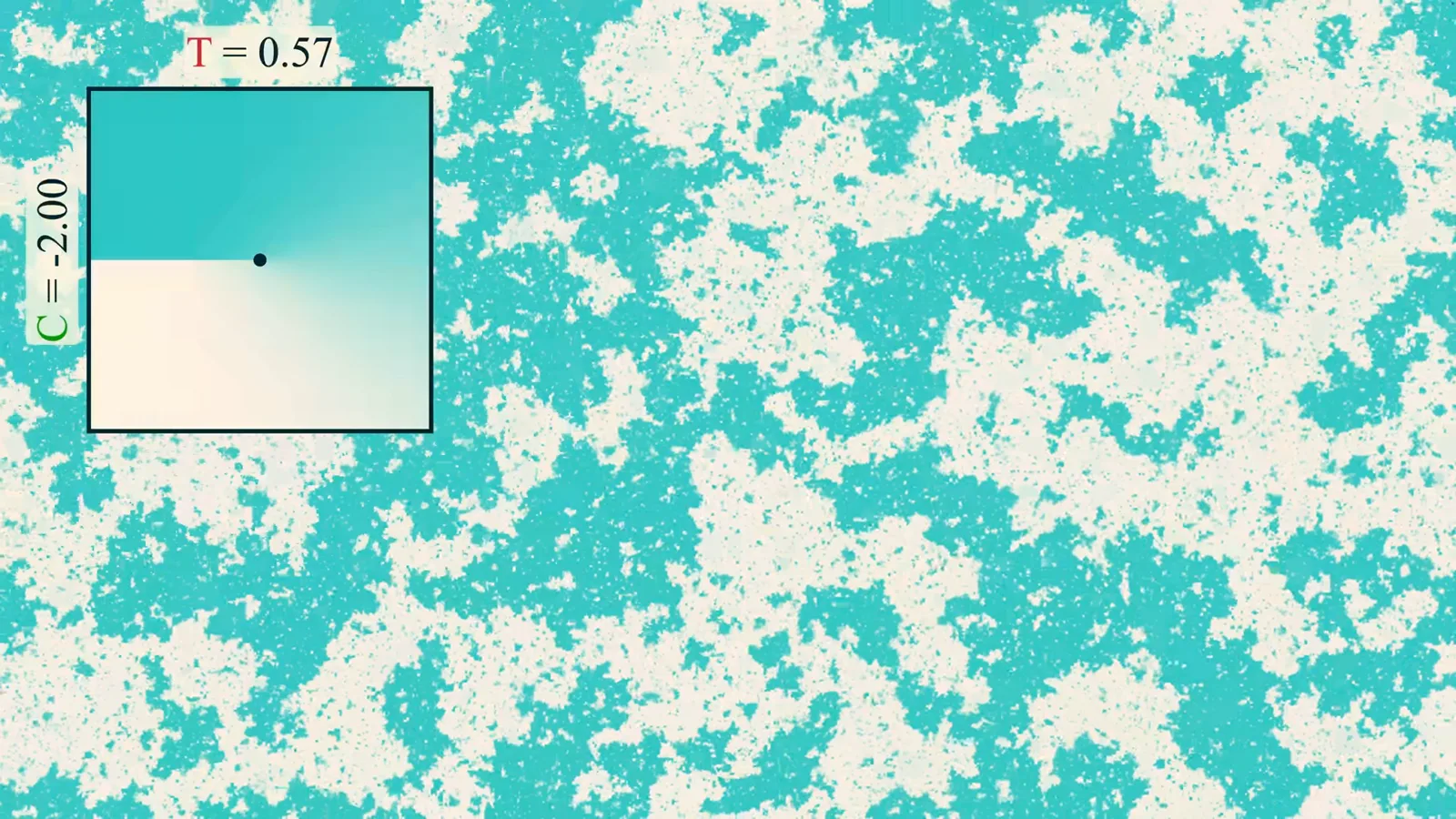
In the simulation, each blue pixel represents a molecule and each white pixel an empty site. Temperature T is one control; the other is chemical potential, which controls particle exchange. The computer array has fixed size, so varying molecule number is easier than changing volume to impose pressure.

Temperature is paired with energy, pressure with volume, and chemical potential with molecule number. Fixing one of these control variables allows its corresponding quantity to fluctuate. Higher chemical potential generally favors more molecules, increasing density somewhat like compressing a fluid.

Temperature controls how strongly energy matters relative to randomness. At high temperature the density changes smoothly as chemical potential varies, like a supercritical fluid. At low temperature, crossing a threshold produces a jump between low-density gas and high-density liquid.

The simulation itself still changes gradually: when the phase transition is underway, liquid-like and gas-like regions coexist, separated by a well-defined interface. To explain why those patterns appear, we need the Boltzmann law.

The Boltzmann law assigns probabilities to molecular configurations, or microstates. This randomness need not come from quantum mechanics: even a deterministic many-particle system is too complicated to track exactly, so a probability distribution can represent our uncertainty about its microscopic state.

Tracking 20 colliding particles might already be difficult, and a teaspoon of water contains roughly 10²³ molecules. Fortunately, we do not need every position and velocity to distinguish water from ice. Macroscopic behavior depends on statistical patterns, not complete knowledge of the microstate.

Treating microstates probabilistically is a useful postulate, though proving that the approximation works in general is a difficult mathematical problem. The distribution gives a configuration x probability proportional to exp(−E(x)/T), using units in which Boltzmann’s constant is one.

A lower-energy microstate has a higher individual weight, but that does not mean the lowest-energy level is always the most likely. We must also count how many microstates have each energy E. If Ω(E) is that set, its total weight is proportional to |Ω(E)| exp(−E/T).

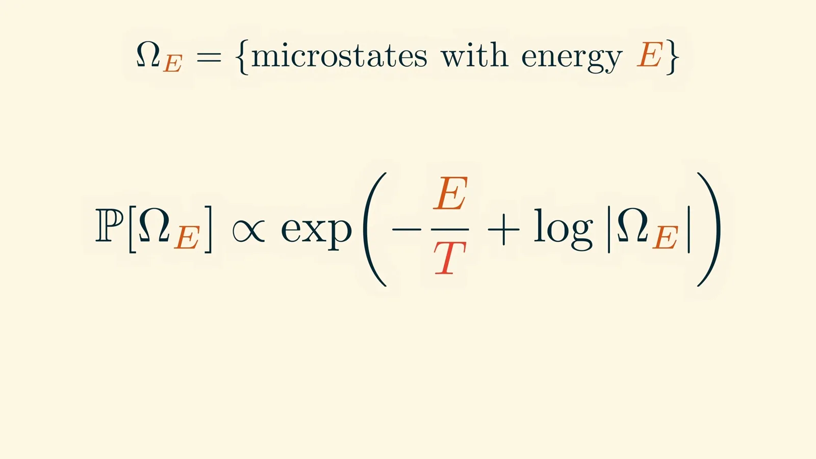
The entropy S(E) is the logarithm of the number of configurations at energy E. The most likely energy level maximizes S − E/T, or equivalently minimizes free energy E − TS. At low temperatures the energy term dominates; at high temperatures the multiplicity represented by entropy matters more.

Consider a fixed number of molecules on a grid. A site holds at most one molecule, and each neighboring pair contributes −1 to the energy. This mimics a preference for nearby molecules while keeping the model simple; kinetic energy is ignored, so the simulation is not a detailed model of real fluid motion.

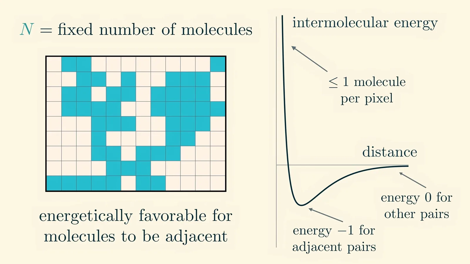
At high temperature, configurations look gas-like: molecules are dispersed, with relatively high energy and many possible arrangements. At low temperature they form a droplet, lowering energy by creating more neighboring pairs, but also reducing entropy because comparatively few arrangements resemble a droplet.

There is no configuration that simultaneously achieves both the lowest energy and the greatest entropy. The competition between these tendencies, controlled by temperature, is central to the phase behavior. We can now ask where the Boltzmann weights themselves come from.

Start with an isolated system at fixed energy and assume its accessible microstates are equally likely. This equal-probability assumption is the starting point for counting configurations, not a consequence of simply knowing the energy alone.

Put two such systems into contact so that they can exchange energy while the combined system remains isolated. The number of combined microstates for a particular energy split is the product of the numbers available to each subsystem, so their entropies add.

If shifting a small amount of energy from one subsystem to the other increases the total entropy, that direction has more compatible combined states. At equilibrium there is no net preferred direction, so the derivatives of the two entropies with respect to their energies are equal.

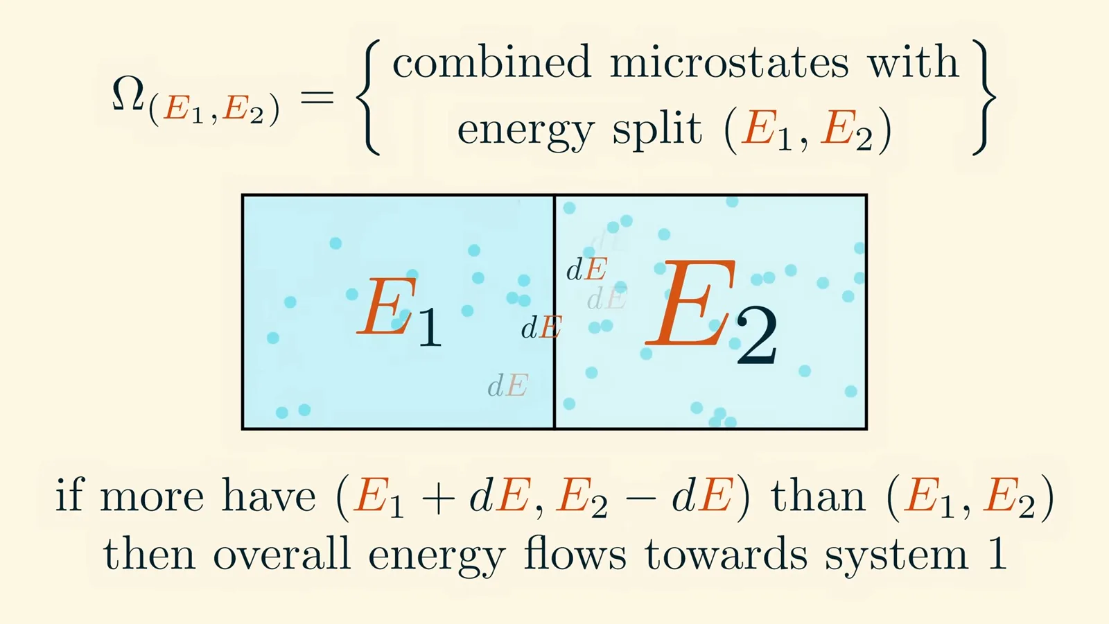
Energy normally flows from hot to cold, whereas it flows toward the larger entropy derivative. Thus the derivative ∂S/∂E is inverse temperature, 1/T in these units. At low temperature a small energy increase opens up relatively more configurations; a hotter system can donate energy to increase total entropy.

To keep a small system at temperature T, place it in contact with a much larger heat bath. Their temperatures equalize, while the reservoir is so large that exchanging energy barely changes its own temperature.

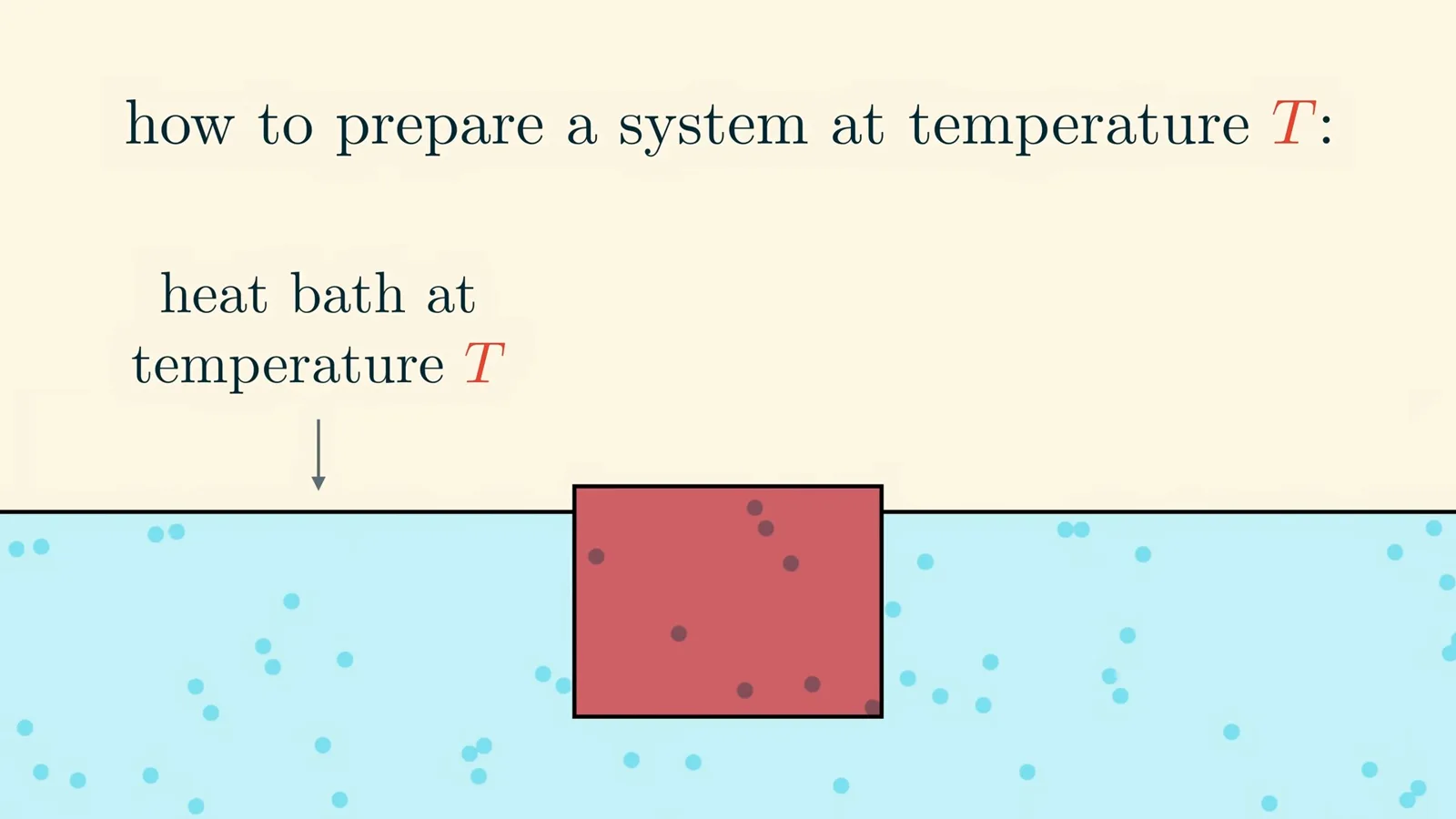
For a particular small-system microstate x, the compatible bath must have total energy minus E(x). Because combined microstates are equally weighted, the chance of x is proportional to the number of compatible bath states, or the exponential of the bath’s entropy at that remaining energy.

The bath’s entropy changes approximately linearly over the relevant energy range, with slope 1/T. The factor independent of x cancels in normalization, leaving P(x) proportional to exp(−E(x)/T). This is the Boltzmann distribution sampled by the simulation.

A formula alone does not make sampling easy: the number of possible configurations grows exponentially. Instead of enumerating them, we can make a sequence of small random changes, analogous to shuffling cards until their arrangement is sufficiently mixed.

For the fixed-particle model, choose two random pixels. If one is occupied and the other empty, consider swapping them. The ratio of the Boltzmann probabilities before and after the swap is Q = exp((E(x) − E(x′))/T), so choose the swapped state with probability Q/(1+Q).

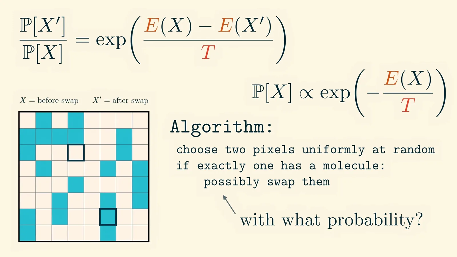
Repeat this step to construct a Markov chain Monte Carlo algorithm known here as Kawasaki dynamics. The energy difference depends only on the nearby pixels, making each step cheap. Given enough steps, the random walk samples approximately from the desired equilibrium distribution.

Swapping only neighboring pixels would look more like physical motion, but typically takes longer to mix. The long-distance swap is a sampling device, not a literal simulation of molecules teleporting. In either version, changing temperature produces dispersed gas-like and clustered liquid-like states over time.

The first model has only temperature as a control. To build a two-dimensional phase diagram without changing the grid’s size, allow particles to pass between the system and a reservoir. The quantity that equalizes when a particular kind of particle can be exchanged is its chemical potential.

For this convention, chemical potential C is −T times the derivative of entropy with respect to particle number. Unlike temperature in this presentation, it can be negative. A system exchanging both energy and particles with a large reservoir has weight proportional to exp((−E + CN)/T).

A positive chemical potential favors configurations with more particles. Now each update can add or remove a molecule at one pixel, rather than swapping two. This single-site approach is Glauber dynamics; careful parallelization makes a larger GPU simulation practical.

The phase diagram maps temperature and chemical potential to density. Above the critical temperature, density varies smoothly; below it, a line separates low-density gas and high-density liquid. This resembles the corresponding region of the water phase diagram even though the model is drastically simplified.

Real molecules move in three dimensions, have complicated shapes and interactions, and possess kinetic energy. The simple model nevertheless reproduces qualitative features of phase change. Universality is the idea that a small number of fundamental ingredients can govern shared large-scale behavior despite different microscopic details.

Below the critical temperature, liquid droplets or gas bubbles form as the phase boundary is crossed. At very low temperature the square lattice makes droplets more square; at higher subcritical temperatures they appear rounder. Their shapes can be studied mathematically using the Wulff construction.

Crossing the boundary slightly may leave the system trapped in the gas-like state. Small droplets shrink before becoming stable, but an artificially inserted droplet above a critical size can grow and transform the system. This long-lived departure from equilibrium is metastability, analogous to supercooled water freezing after a disturbance.

At the critical point, clusters appear on many scales and the image has approximate self-similarity under coarse-graining. Away from the critical point, zooming out instead produces a more uniform picture. Winstein mentions the critical-brain hypothesis as a speculative connection beyond the lesson’s scope.

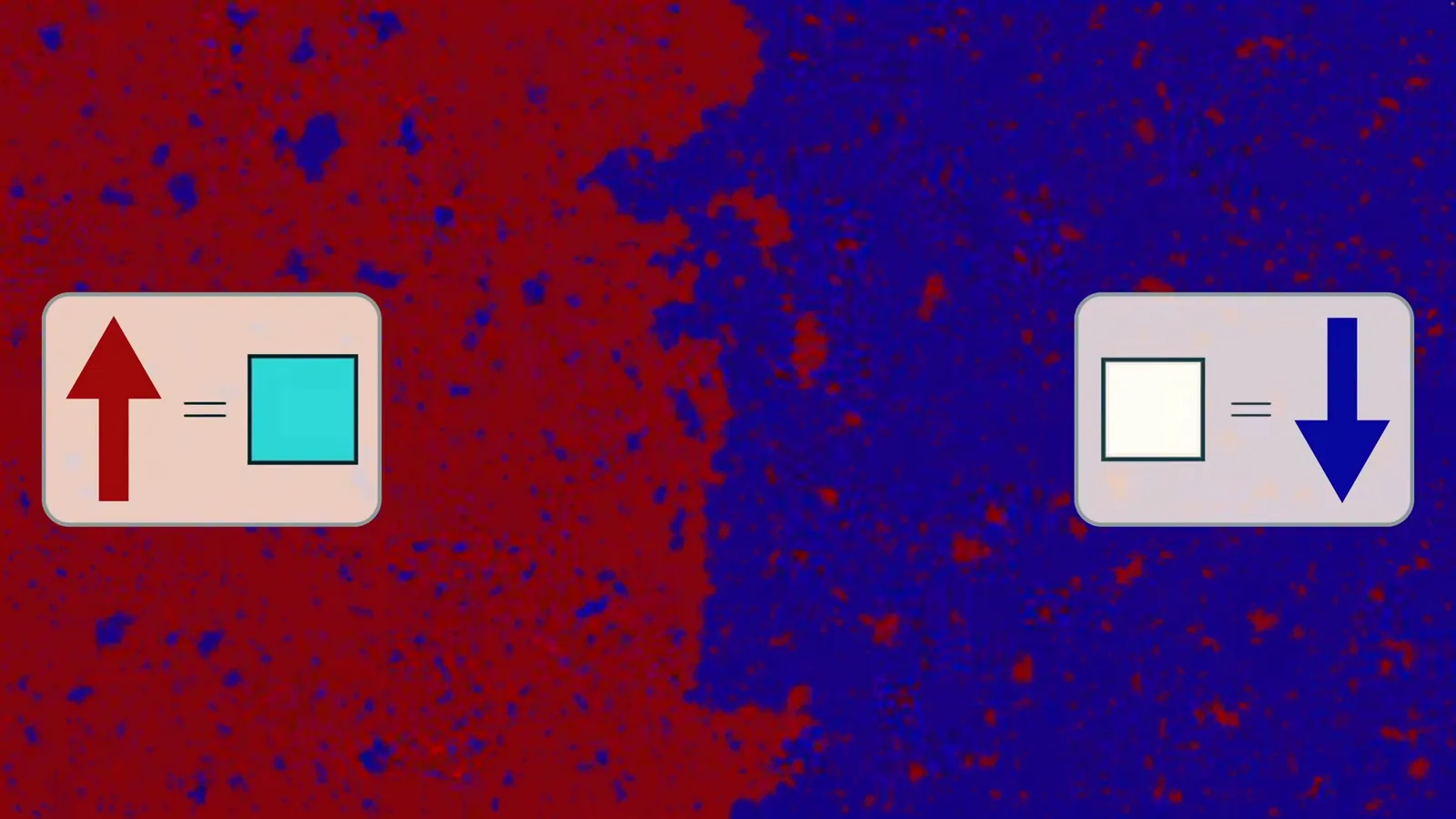
The liquid–vapor lattice is also an Ising model of a magnet: identify an occupied site with an up spin and an empty site with a down spin, and reinterpret chemical potential as an external magnetic field. Fixed opposing spin directions at the borders are Dobrushin boundary conditions.

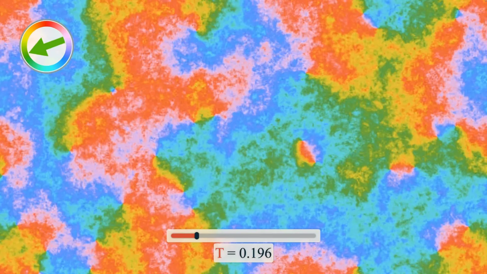
If spins can point in any direction in a plane, the related XY model behaves differently in two dimensions. Its colored direction field can form vortices of opposite orientations: opposite types attract and like types repel, in an analogy to electrical forces.

These models can also be studied in higher dimensions and other geometries. Even the three-dimensional version of the simple liquid–vapor model is much less completely understood: unlike in two dimensions, the critical temperature is known numerically rather than by the same exact formula.

A rigorous microscopic model of real water would need to account for molecular geometry, electrical asymmetry and free motion in three dimensions. Mathematics often gains understanding by simplifying a system while keeping the features that matter. The follow-up video simplifies the lattice model further to show rigorously how its phases arise.