How Laplace Transforms Explain a Driven Oscillator

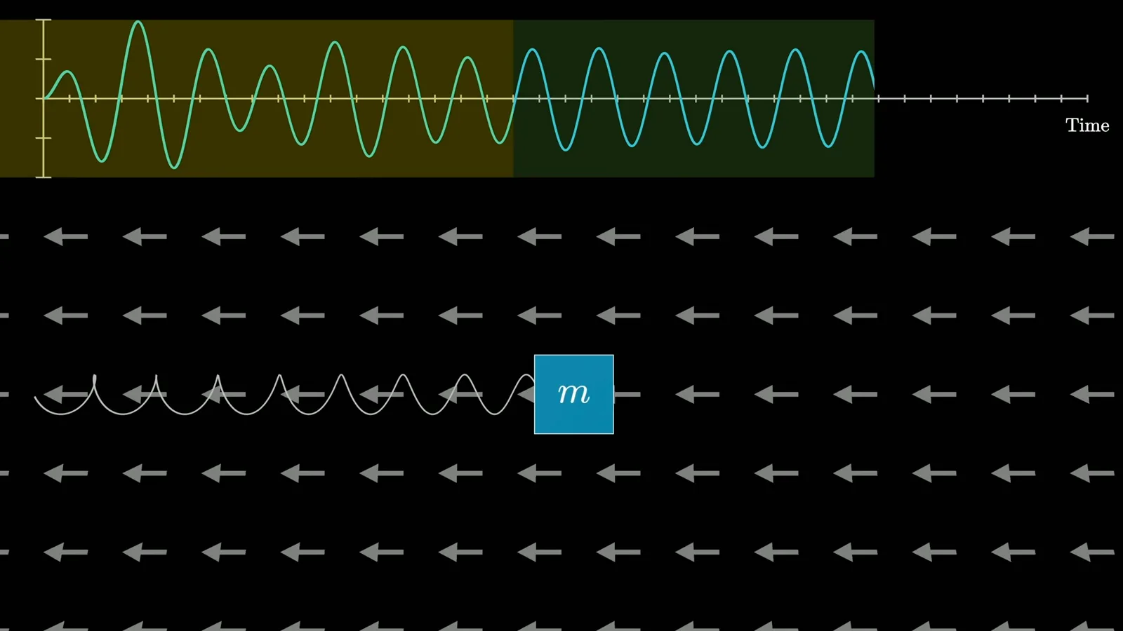
Imagine a mass on a spring, pushed by an external force that oscillates at a frequency unrelated to the spring’s natural frequency. The motion initially grows and shrinks irregularly, then settles into a rhythm. Can we predict the startup motion, how long it lasts and the size of the eventual swings?

The previous chapters introduced the complex s-plane. Each point s represents an exponential e^(st): the imaginary part governs oscillation, while the real part determines growth or decay. Many physical motions can be understood by breaking them into such exponential pieces.

A Laplace transform turns a function of time into a function of the complex variable s. In the kinds of examples considered here, poles of the transformed function reveal exponential pieces of the original. Specifically, e^(at) transforms to 1/(s−a), where the defining integral converges for Re(s) > Re(a).

The transform is linear: transforming a weighted sum gives the same weighted sum of transforms. Thus a sum of exponentials becomes a sum of fractions, with poles corresponding to the constituent exponentials. Imaginary parts suggest oscillation; negative real parts indicate decay, while positive real parts signal growth.

In physics we often know a differential equation without knowing its solution. The transform can take us directly from that equation to a transformed solution, which is valuable both as a step toward a formula and as a representation of the system’s dynamics.

The crucial third rule is ℒ{f′}(s) = sF(s) − f(0). Differentiation in time becomes multiplication by s, with a correction for the initial value. That correction may seem untidy, but it automatically carries an initial condition into the algebra.

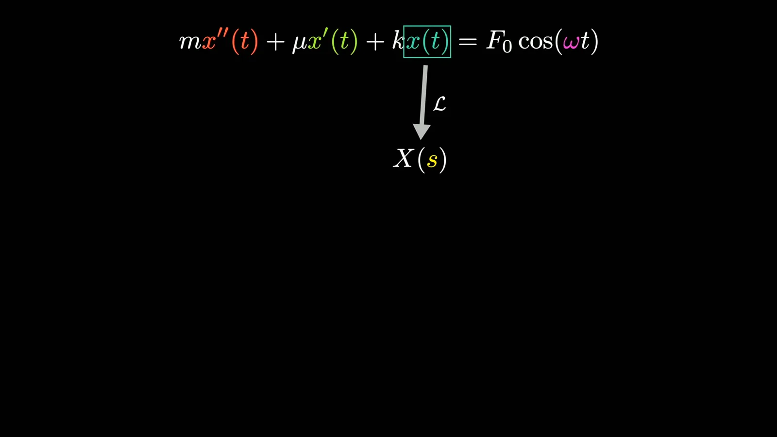
Consider a spring whose restoring force is −kx and whose damping force is proportional to velocity. Add a periodic external force F₀ cos(ωt), like wind blowing alternately in opposite directions. The frequency ω need not equal the spring’s own frequency.

The resulting equation is m x″ + μx′ + kx = F₀ cos(ωt). It is still linear, but it is now driven: the right-hand side is nonzero. Similar mathematics appears in the channel’s discussion of light driving charges in a material.

Write X(s) for the transform of x(t), x₀ for its initial position and v₀ for its initial velocity. The derivative rule gives ℒ{x′} = sX − x₀. Applying it again gives ℒ{x″} = s²X − sx₀ − v₀, so both initial conditions enter the transformed equation.

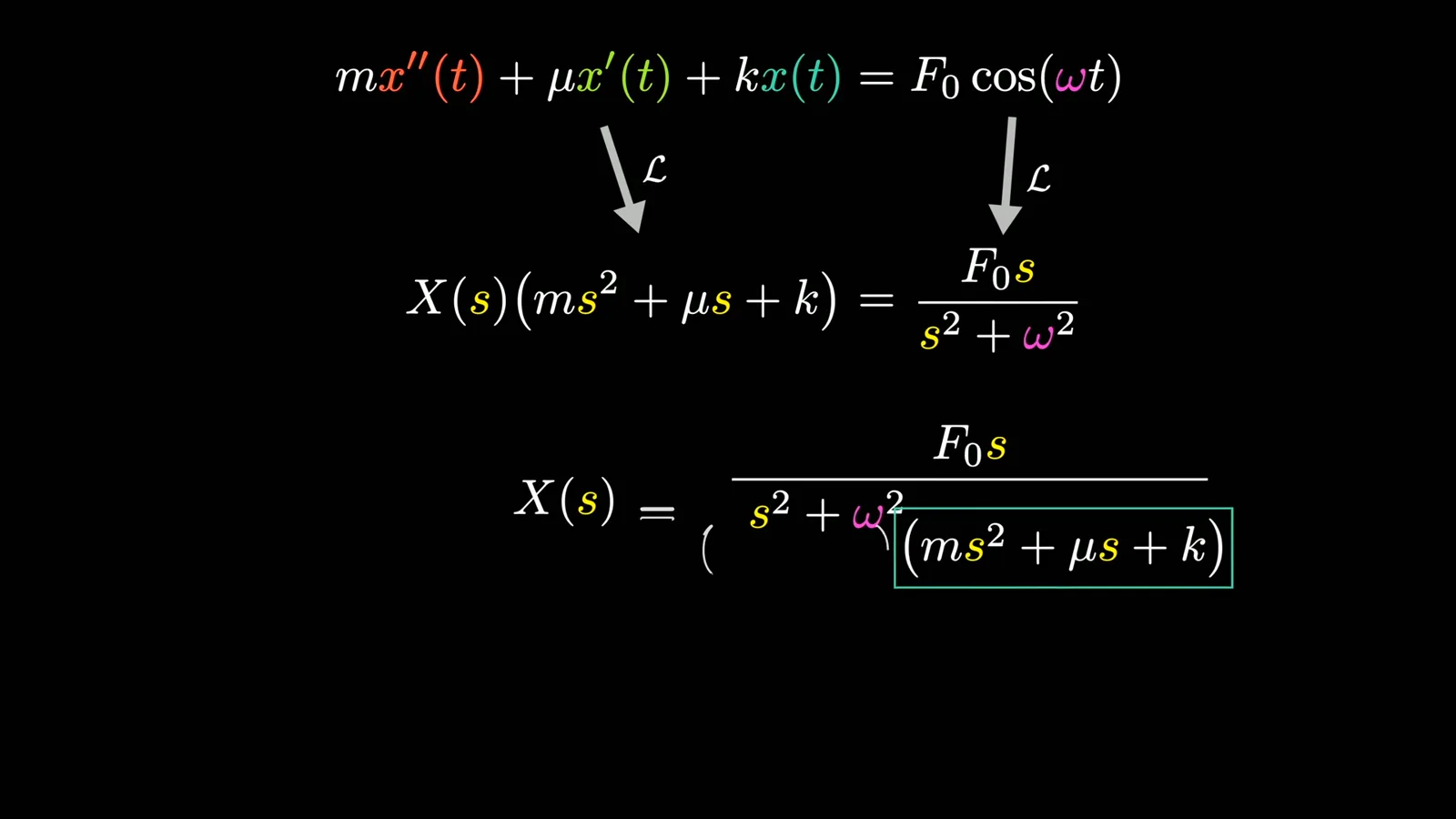
The terms multiplying X combine into the polynomial ms² + μs + k. For a cleaner first example, suppose x₀ = v₀ = 0. The derivatives have now become powers of s, leaving an equation that can be manipulated algebraically.

The transform of cos(ωt) is s/(s² + ω²). The denominator has roots at ±iω, reflecting the forcing’s oscillation. Dividing by the oscillator polynomial gives X(s) = F₀s/[(s² + ω²)(ms² + μs + k)] for the zero-initial-condition example.

Before inverting X, inspect its poles. The roots of ms² + μs + k represent the natural motion; for positive mass, stiffness and damping they have negative real parts. When damping is small enough for the underdamped case, they also have imaginary parts, indicating oscillation that fades.

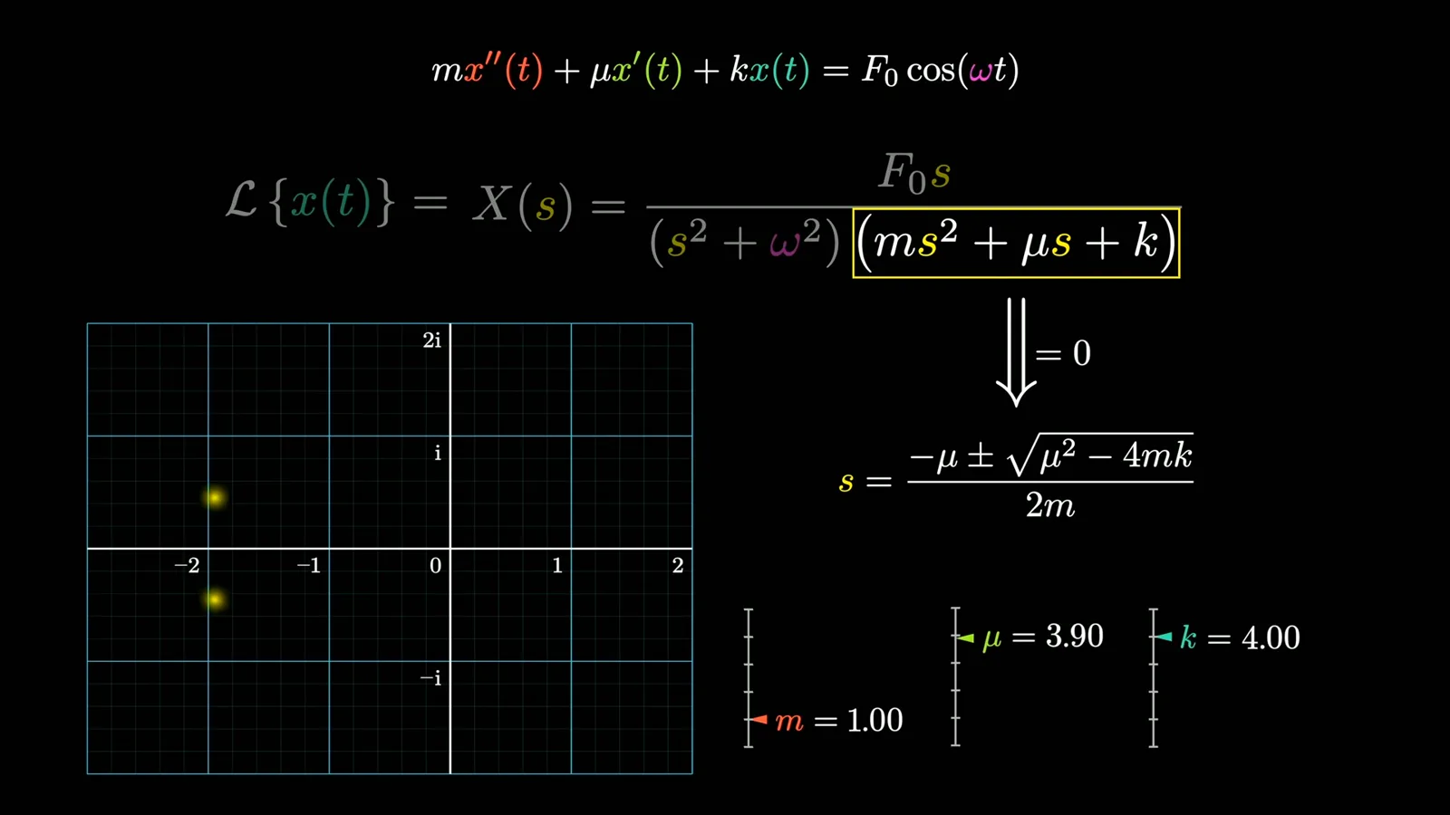
The other two poles, at ±iω, come from the driving force and describe sustained oscillation at its frequency. Think of pushing a swing at a frequency different from its natural one: once transients die away, the enduring response follows the forcing frequency.

The simulation makes the distinction visible. The irregular startup is the sum of a decaying natural component and the continuing forced component. As the former fades, the latter remains as a steady sinusoid, generally with a phase shift relative to the force.

To find an explicit expression, use partial fraction decomposition. When the four poles are distinct and uncancelled, X can be written as a sum of terms with denominators s minus a pole. Each term inverts to an exponential whose exponent is that pole, multiplied by its coefficient. Repeated poles require a modified decomposition.

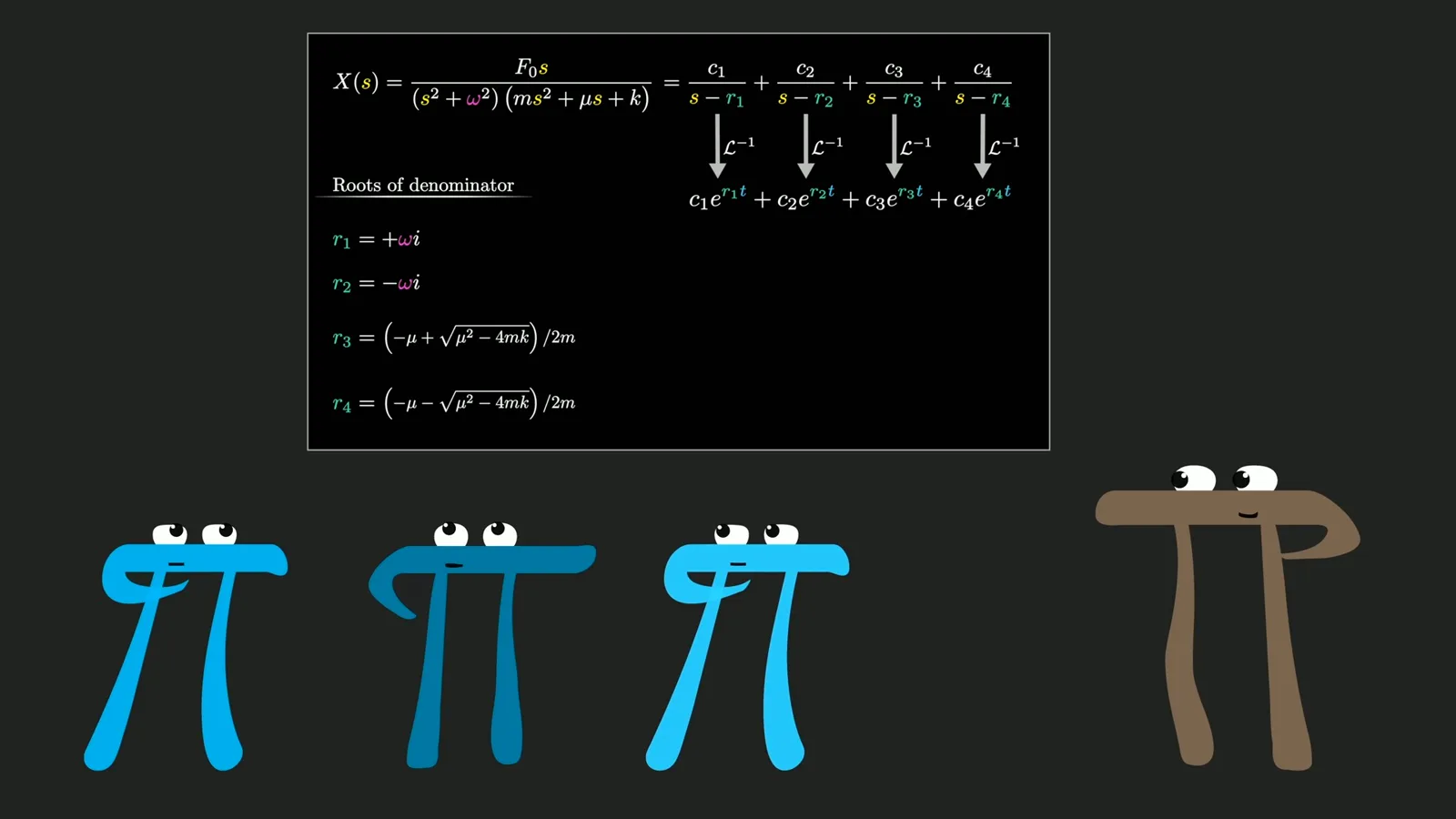
The coefficients of the two forcing terms combine into the steady oscillation. In the small-damping approximation shown in the video, their form invites an examination of how response amplitude changes as the driving frequency approaches the spring’s resonant frequency. Damping matters when analyzing the response near resonance.

This is the broad strategy: transform the differential equation, solve the resulting algebraic equation, inspect the poles and invert if an explicit time-domain answer is needed. The whole procedure depends on the derivative rule.

First test that rule on f(t) = e^(at). Its derivative is ae^(at), so linearity gives a/(s−a). A small algebraic rearrangement gives s/(s−a) − 1, exactly sF(s) − f(0), since f(0) = 1.

Linearity extends this check to finite combinations of exponentials. That is useful intuition, though it is not a general proof. The familiar textbook proof starts from the defining Laplace integral and applies integration by parts, under conditions that make the boundary term at infinity vanish.

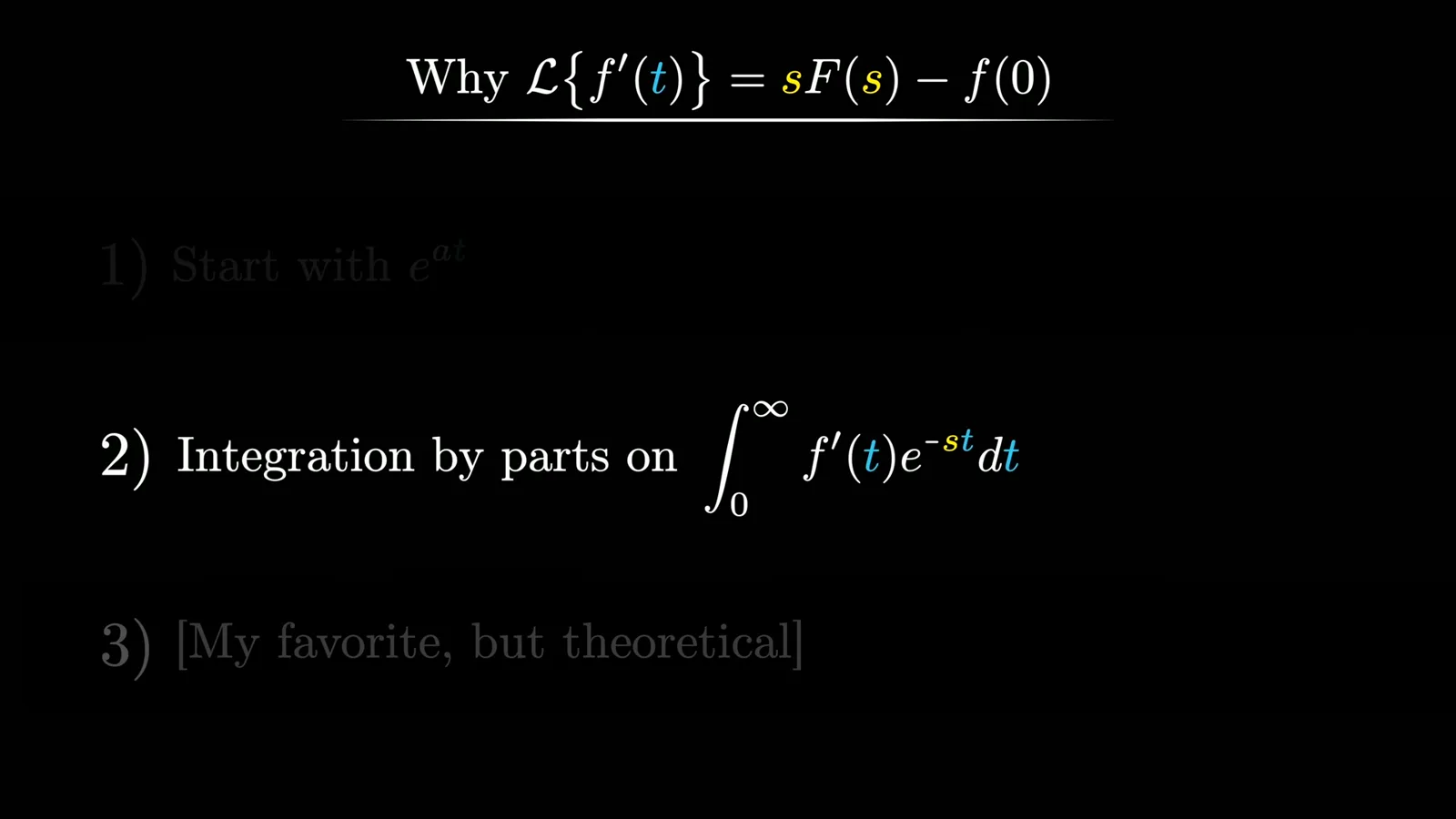
Integration by parts is concise, but the speaker finds it less illuminating about why multiplication by s and the initial condition fit the transform’s purpose. A third explanation relies on the inverse Laplace transform, which has not yet been developed.

The inverse matters beyond cases that break neatly into simple fractions: what if the original function is not a discrete sum of exponentials? The next chapter will explore inversion, contour integrals and the relationship with Fourier transforms, building the transform and its inverse together.