Hilbert’s Curve: What an Infinite Path Reveals About Finite Images

Can an infinite mathematical construction tell us anything useful about a finite problem? Imagine converting a camera image into sound so that a listener could learn to recognize shapes. Each pixel might control a frequency, with brightness represented by volume.

The difficult choice is how to assign frequencies to positions. If neighboring pixels have neighboring frequencies, a recognizable feature might produce a more coherent pattern of sound. This is a thought experiment, not a demonstrated sensory device.

A path through the image gives us an ordering: follow it from low to high frequencies, assigning a frequency to each pixel as we go. We want successive points on the path to lie close together in the image.

The first path I will build is a finite approximation to the Hilbert curve. Its winding shape may look complicated, but its construction follows a simple recursive rule.

Start with a U-shaped route through four positions. To make a finer route, put a copy in each of four quadrants, rotate the copies as needed, and connect them. Repeat the same operation to obtain finer grids.

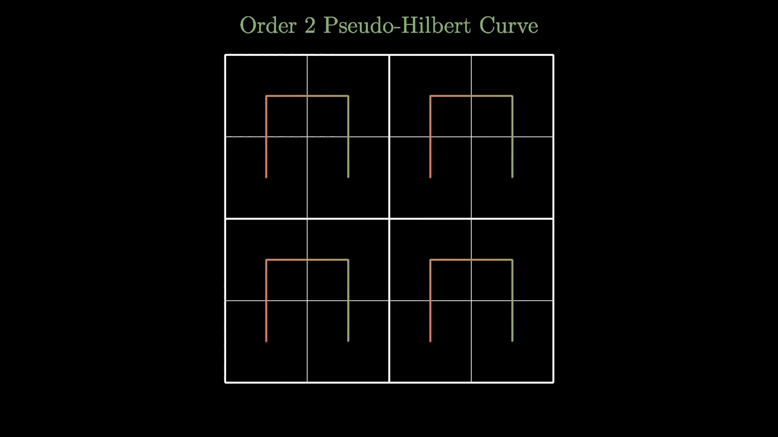
At order n, the grid has 2ⁿ positions on each side. An order-eight approximation therefore visits the pixels of a 256 by 256 grid. Each finite path has a definite resolution and visits a finite number of pixel locations.

Why use this ordering instead of a simple row-by-row snake? Both paths can move between neighboring pixels, but their behavior as we increase the resolution differs. Imagine keeping the frequency assigned to a point fixed while refining the image.

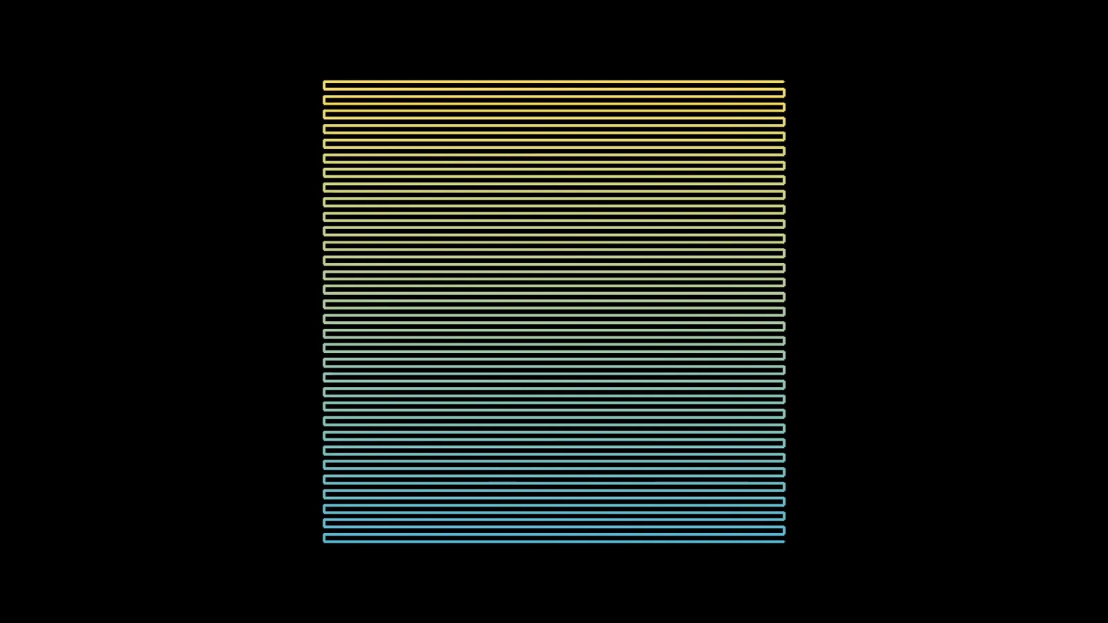
For the row-by-row path, refining the grid can send the same relative position along the path to a distant horizontal location. A small change in resolution may therefore change the sound assigned to a visual feature substantially.

The recursive Hilbert approximations behave more stably: at a fixed relative position along the path, successive locations settle into smaller regions as the grid is refined. That makes the ordering attractive for a gradual increase in detail.

This locality has a direction. Nearby inputs along the path map to nearby positions in the square; it does not mean that every pair of neighboring pixels must be adjacent in the one-dimensional ordering.

The history goes back to Giuseppe Peano, who described a space-filling curve in 1890, and David Hilbert, who gave another construction in 1891. The startling claim is that a continuous curve can reach every point of a square.

A finite drawing only suggests the idea. No finite grid path visits every point of a continuous square. The space-filling curve is the limit of the sequence of increasingly fine approximations, not any one drawing in the sequence.

Mathematically, the result can be expressed as a continuous map from the interval [0, 1] onto the square [0, 1]². Different inputs can reach the same output, so filling the square does not require a one-to-one correspondence.

What does continuous mean here? If two input values are sufficiently close, their output points must be as close as we choose. In the familiar epsilon-delta formulation, every desired output tolerance has a corresponding input tolerance.

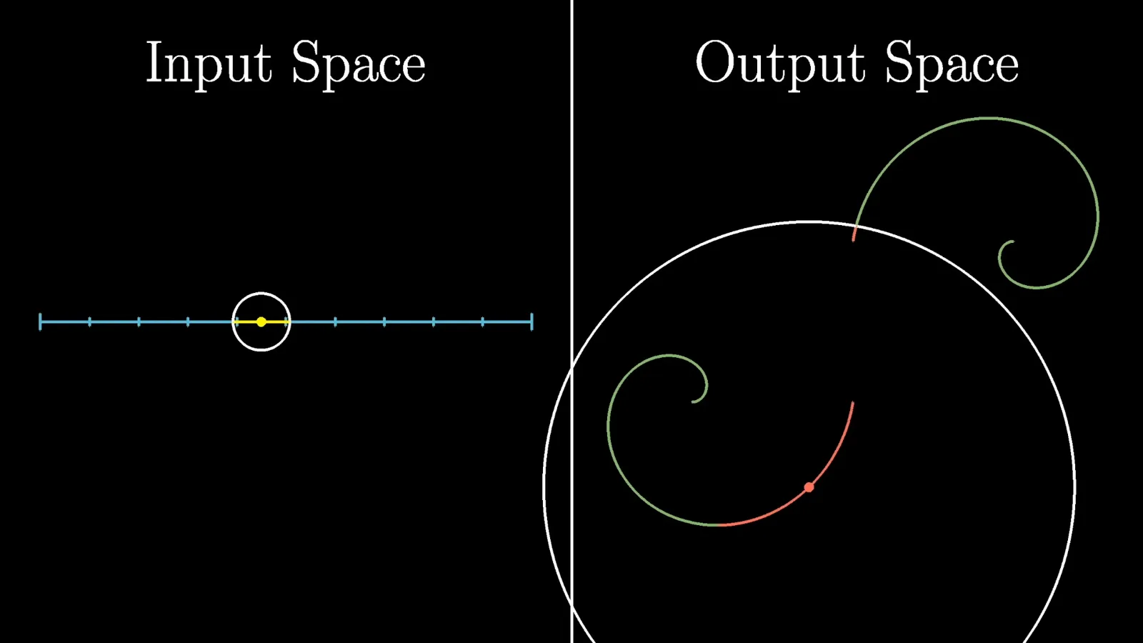
Continuity rules out jumps, but it does not prohibit the path from folding and revisiting places. Our ordinary picture of a smooth, finite-length line can mislead us when applied to this limiting object.

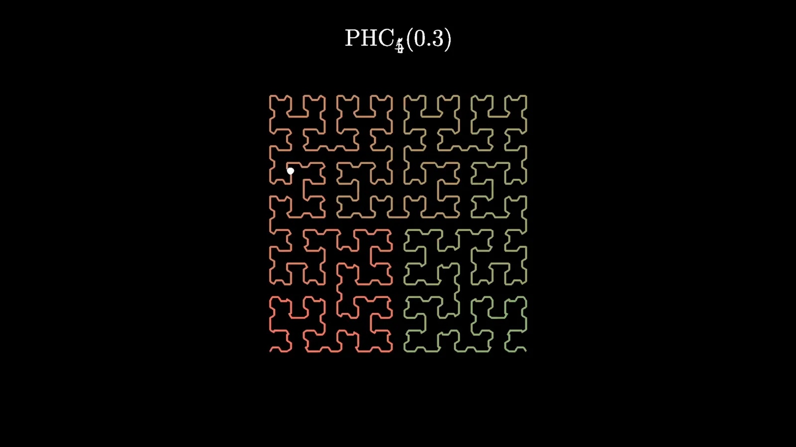
To define the limit, fix one input along the interval and look at its output in each successive approximation. The recursive construction keeps those outputs in successively smaller regions, so their positions approach a limiting point.

Do this for every input, and the limiting points define a candidate function. Showing that the function is well defined, continuous, and reaches every point of the square requires arguments about the construction; pointwise convergence alone does not prove all those properties.

The same idea can be extended beyond one square. Arrange a route through successive squares in the plane and connect suitably scaled or translated space-filling pieces. With an unbounded input interval, the construction can reach the whole plane.

The surprising infinite object also illuminates the finite example. We do not need infinitely many pixels or an infinitely long computation to use a finite approximation. The useful insight is the stable recursive pattern shared by successive resolutions.

Infinite mathematics can expose structure that is hard to see in a single finite drawing. In this case, the limiting curve makes the refinement behavior precise, while the practical audio mapping remains a proposal to investigate.