Making GPU Training Faster: Pipelines, Fusion and Custom Kernels

Corwin and a second speaker introduce a talk about efficient GPU training. CPUs excel at low-latency sequential work, while GPUs provide enormous parallel throughput. The question is how to organize machine-learning workloads to benefit from that throughput.

Corwin uses a deliberately provocative comparison: a single floating-point operation can be much slower when sent to a GPU than on a CPU, because GPU execution has overhead. That is not a realistic GPU workload. Matrix multiplication, by contrast, can divide substantial work across many threads.

In the example, a 2048-by-2048 matrix multiplication takes about 28 milliseconds on a CPU and 200 microseconds on a GPU. The illustrative measurements reverse the single-operation comparison: sufficient parallel work makes the GPU dramatically faster.

The second speaker reviews training: feed inputs through a model, compare outputs with targets to calculate a loss, compute gradients with respect to the parameters, and take a small step that reduces the loss. Repeat this process thousands or millions of times.

PyTorch provides GPU kernels and automatic differentiation. A data loader supplies batches; the model computes outputs and loss; backward computes gradients; and the optimizer updates parameters. Moving the model, inputs and targets to the GPU places the expensive forward and backward work there.

Corwin explains the CPU–GPU pipeline. The CPU prepares data and submits kernel launches, including parameters sent through the driver. The GPU executes the operations, such as a linear layer followed by ReLU. A kernel is roughly a function implementing a GPU operation.

A naïve timeline would leave the GPU idle while the CPU prepares every operation. In practice launches are asynchronous: the CPU can queue the next kernel and prepare the next batch while the GPU works on earlier operations. The queue lets useful CPU and GPU work overlap.

A profiler such as NVIDIA Nsight Systems shows CPU-side CUDA API calls and GPU hardware activity. Corwin looks for gaps in the GPU activity bar as a starting point: idle time means the device is waiting instead of doing useful work.

Copying results back to the CPU can force synchronization. The CPU waits for queued GPU work and the transfer, draining the pipeline; subsequent data preparation can then become visible as GPU idle time. The cost depends on what follows the synchronization, not just the synchronization itself.

An explicit output.cpu() for metrics is an obvious synchronization. A more subtle one is a Python if that converts a GPU tensor, such as an is-NaN result, to a Boolean: the CPU must know the answer before choosing a branch. The tensor operation alone is not necessarily the synchronization.

An audience member suggests the optimizer step might need synchronization to reload weights. Corwin explains that weights can stay on the GPU and optimizer operations can launch GPU kernels, so a CPU-side call does not necessarily imply a transfer or a synchronization.

The demonstrated CPU-to-GPU copy can also block. The source memory must remain available while the GPU reads it, and the default transfer behavior in the example waits for completion. Very small transfers may behave differently, but the important point is to inspect the actual pipeline.

A short synchronization is not necessarily expensive if the CPU immediately resumes launching work. It becomes particularly harmful when costly preparation of the next batch follows it, because that preparation can no longer overlap earlier GPU computation.

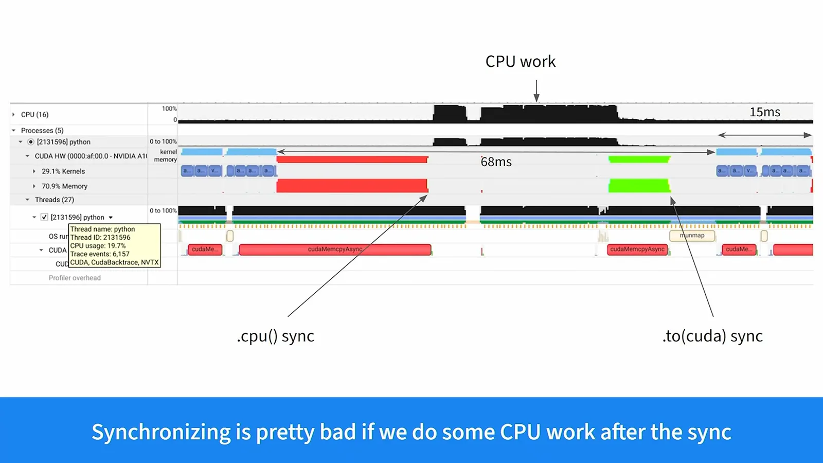
One remedy is to accumulate metrics on the GPU and copy them back only occasionally. A NaN check can be handled asynchronously, for example by a separate CPU thread, allowing the main thread to keep launching kernels. This changes behavior: some extra work may run before the failure is acted on.

For asynchronous host-to-device transfers, pinned host memory allows direct memory access without paging the source out. The example uses non_blocking=True as well. The programmer must manage the source’s lifetime and avoid modifying it while the transfer is in flight.

Even after those synchronizations are removed, copies may still leave gaps; overlapping transfers with computation is possible but requires more careful code. A full GPU activity bar only means the GPU is busy, not that the kernels themselves use its resources efficiently.

A simplified GPU consists of many streaming multiprocessors, or SMs, each with compute resources, registers and shared memory for cooperating threads. An H100 in the example has 132 SMs. Efficient kernels divide a problem into chunks that can largely be processed independently, then combine or store results.

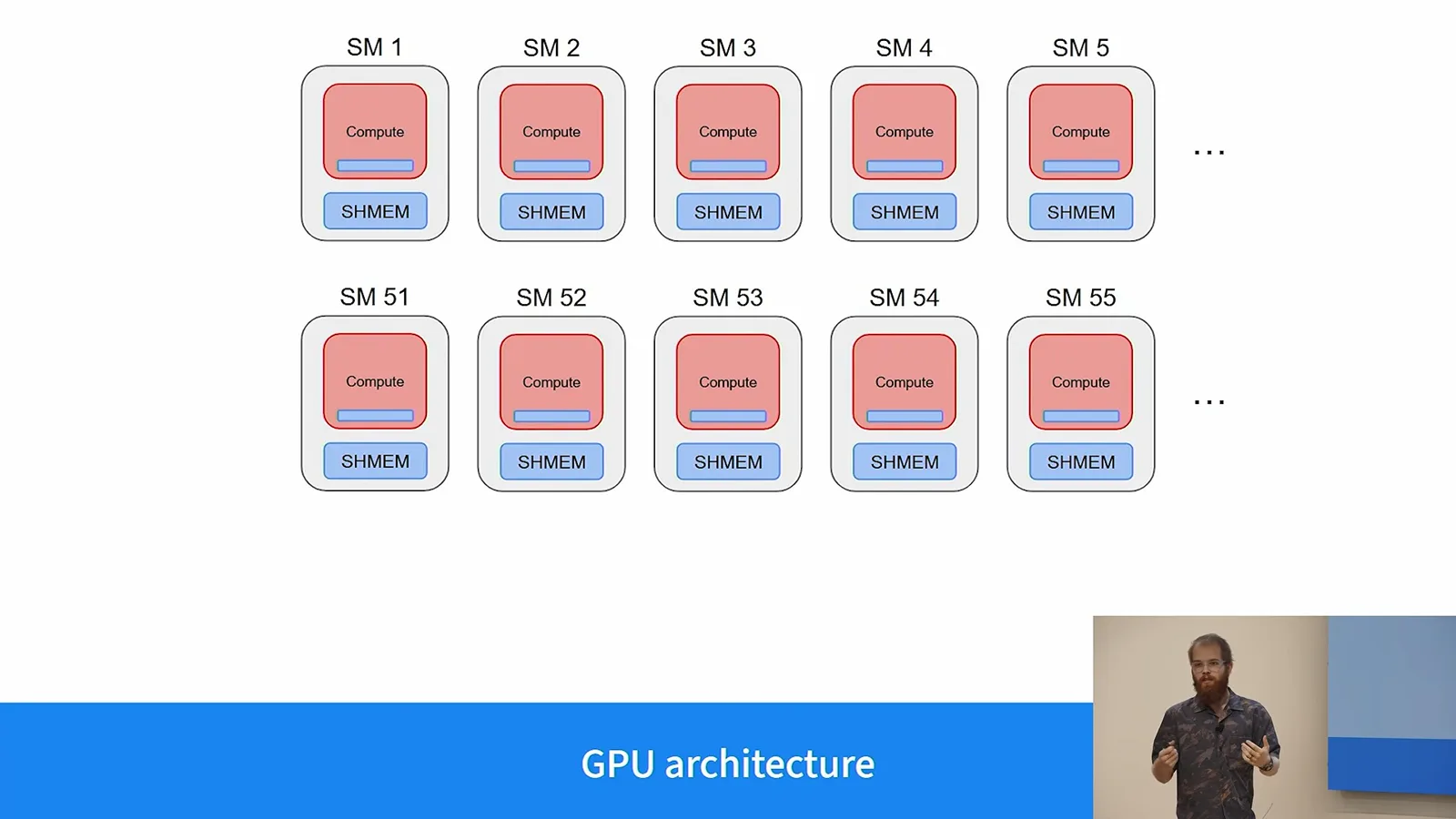
Global memory supplies inputs and stores outputs, with L2 cache shared between SMs. The talk gives approximate H100 bandwidths of 3 TB/s for global memory, 7 TB/s for L2 and 26 TB/s for shared memory. The hierarchy makes reuse of data close to computation important, subject to capacity and access constraints.

The main bottlenecks are computation, memory traffic and kernel-launch overhead. CPU launches can take roughly 5–10 microseconds in the example, so a succession of tiny GPU kernels can starve the device even though each operation itself is quick.

The second speaker outlines remedies. Tensor cores accelerate suitable compute-heavy operations such as matrix multiplication. Kernel fusion can reduce memory traffic and amortize launch overhead, while CUDA graphs can record and replay sequences of small kernels to reduce repeated launch overhead.

Consider layer normalization, ReLU and an addition in a skip connection. If separate kernels repeatedly store intermediate results to global memory and load them again, memory traffic dominates. A fused kernel can load data, perform several operations, then store the final result.

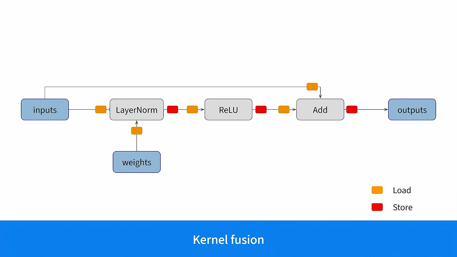
Writing a separate fused kernel for every combination is impractical. torch.compile traces a model, looks for fusion opportunities and can benchmark alternatives. The initial compilation is slow, but subsequent executions can benefit from the resulting kernels.

Graph breaks reduce fusion opportunities. The speakers mention unsupported Python constructs, custom operators and accidental CPU–GPU synchronization as possible causes. Compiling with fullgraph=True can expose breaks rather than silently splitting the graph.

For a concrete custom-kernel example, the speaker wants to sum many tensors to log mean gradients. A Python loop launches many small reductions sequentially. In the profile, the CPU takes around five microseconds to enqueue a kernel that can run in less than one microsecond, leaving the GPU waiting.

torch.compile does not solve this example automatically and can even be slower. It traces the unrolled loop rather than discovering the desired parallel work decomposition; when fusion is limited, generated kernels may not outperform highly optimized library kernels. A custom kernel can express the parallelism directly.

The proposed decomposition assigns one tensor to a thread block, with blocks scheduled dynamically on SMs. Thousands of tensors can still be handled by 132 SMs: as an SM finishes one block, it can take another, so different tensor sizes can balance over time.

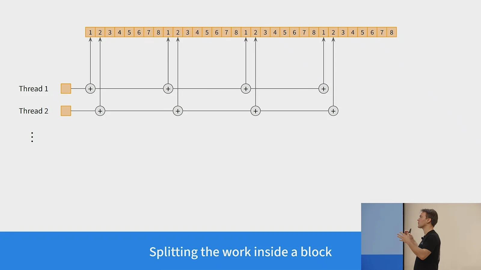
Within a block, threads compute partial sums and then reduce them together. Neighboring threads read neighboring memory locations so their accesses can be combined efficiently. The final result is written to global memory.

The CUDA example launches one block per tensor with 1,024 threads per block. blockIdx selects the tensor, and threadIdx selects a thread’s starting element. Each thread processes elements at a stride of the block size, then the block reduces its partial sums.

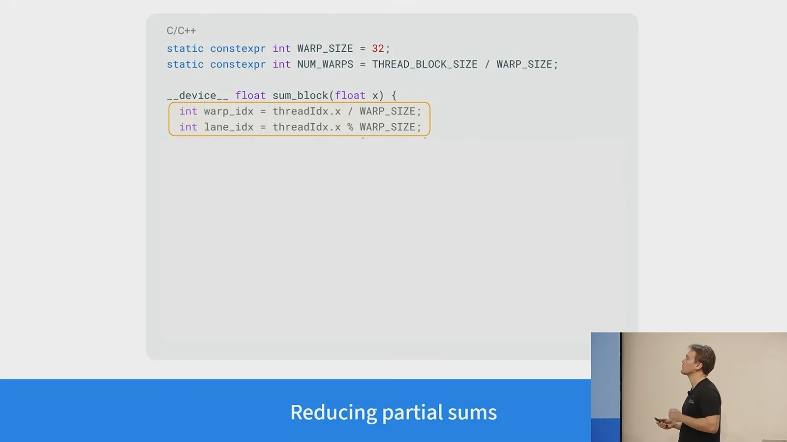
Threads execute in warps of 32. The code first reduces within each warp, uses shared memory for one partial result per warp, and synchronizes the block so every warp’s result is available. A final warp reduction combines those results; thread zero stores the answer.

The reported example improves from roughly 20 milliseconds to 30 microseconds, nearly a thousandfold. The speaker cautions that writing such a kernel may take a beginner a week or an experienced developer an afternoon; the payoff depends on the workload.

Asked which language to use for custom kernels, the speaker recommends first trying clearer or vectorized PyTorch. Triton is usually the next step; CUDA is useful when Triton cannot express the kernel or maximum performance matters. The team rarely writes a whole kernel in PTX, though it may insert an individual instruction.