Newton’s Method and the Fractal Boundaries Between Roots

Newton’s fractal is not just an intricate picture: its shape reveals surprising behavior in a practical root-finding algorithm. The goal is to understand why the boundaries are complicated, not merely admire the pattern.

A root of a polynomial is an input where its output is zero. That task appears throughout engineering. In computer graphics, for example, rendering a mathematical curve requires deciding which pixels lie close enough to it to be colored.

Fonts and vector graphics are often described by Bézier curves rather than pixels. To draw a stroke, we need the distance from a pixel to the curve. We could sample many points, but that approach can be inefficient and imprecise.

Parameterize the curve by t. The squared distance from a fixed pixel to the curve is a polynomial in t. To find an interior minimum, differentiate and find where the derivative is zero, while also checking the endpoints of the allowed parameter interval. This reduces part of rendering to polynomial root finding.

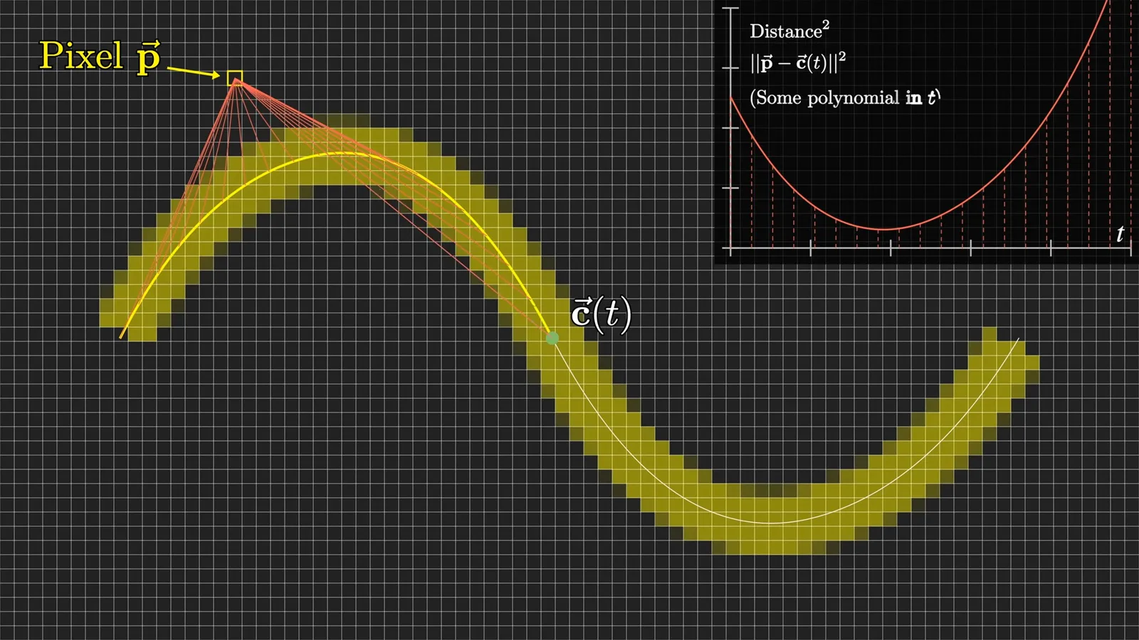
The quadratic formula solves degree-two equations, and there are formulas for cubics and quartics. There is no general formula in radicals for arbitrary polynomials of degree five or higher. Numerical methods can nevertheless approximate roots when their conditions for convergence are met.

Newton’s method starts from a guess x₀. Draw the tangent to the graph at that point and use the place where the tangent crosses the x-axis as a better guess: xₙ₊₁ = xₙ − P(xₙ)/P′(xₙ). The update requires a nonzero derivative.

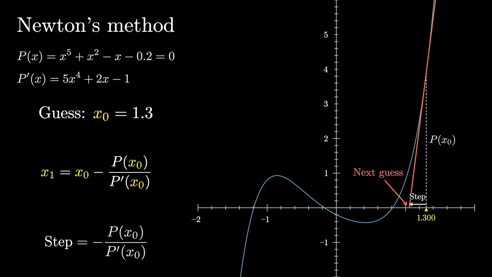
Repeat the operation: evaluate the polynomial and derivative at the new guess, draw the new tangent and find its intercept. In a favorable example, the guesses rapidly approach a root. If the function value is large the step grows; if the slope is steep, the same height calls for a smaller step.

Newton used a version of the method, and Joseph Raphson published a simpler formulation, hence the name Newton–Raphson method. Approximating square roots by hand is a useful way to practice the iteration.

A good starting point near a root often converges quickly, but a distant guess can behave poorly. In the example, guesses bounce around a local minimum above the axis; local tangent approximations there say little about the distant real root. An iteration can also encounter a zero derivative or fail to converge.

Now allow complex starting values. A degree-five polynomial has five complex roots counted with multiplicity, by the fundamental theorem of algebra. Although a real graph and its tangent no longer give the same picture, the same update finds the zero of a local linear approximation in the complex plane.

Run the iteration from many starting points at once. Most shown points settle near one of five roots, while others wander for many steps. Color each starting point by the root it approaches, then put it back in its original location.

Increasing the resolution exposes elaborate boundaries between the colored basins. Near such a boundary, an extremely small change in the initial guess can send the iteration to a different root. This sensitivity is a property of the algorithm’s dynamics, not decoration added to the picture.

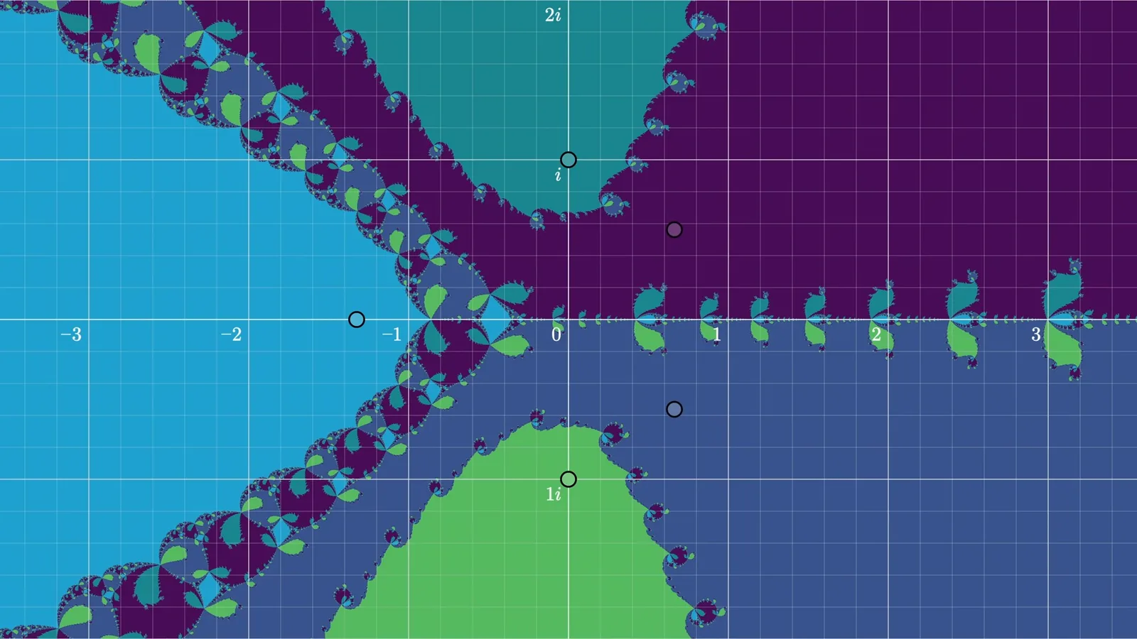
Move the roots and the shape changes, but the examples retain complicated boundaries. Near each root there is a region whose starting points converge to it. The sensitive behavior is concentrated around the boundaries between basins.

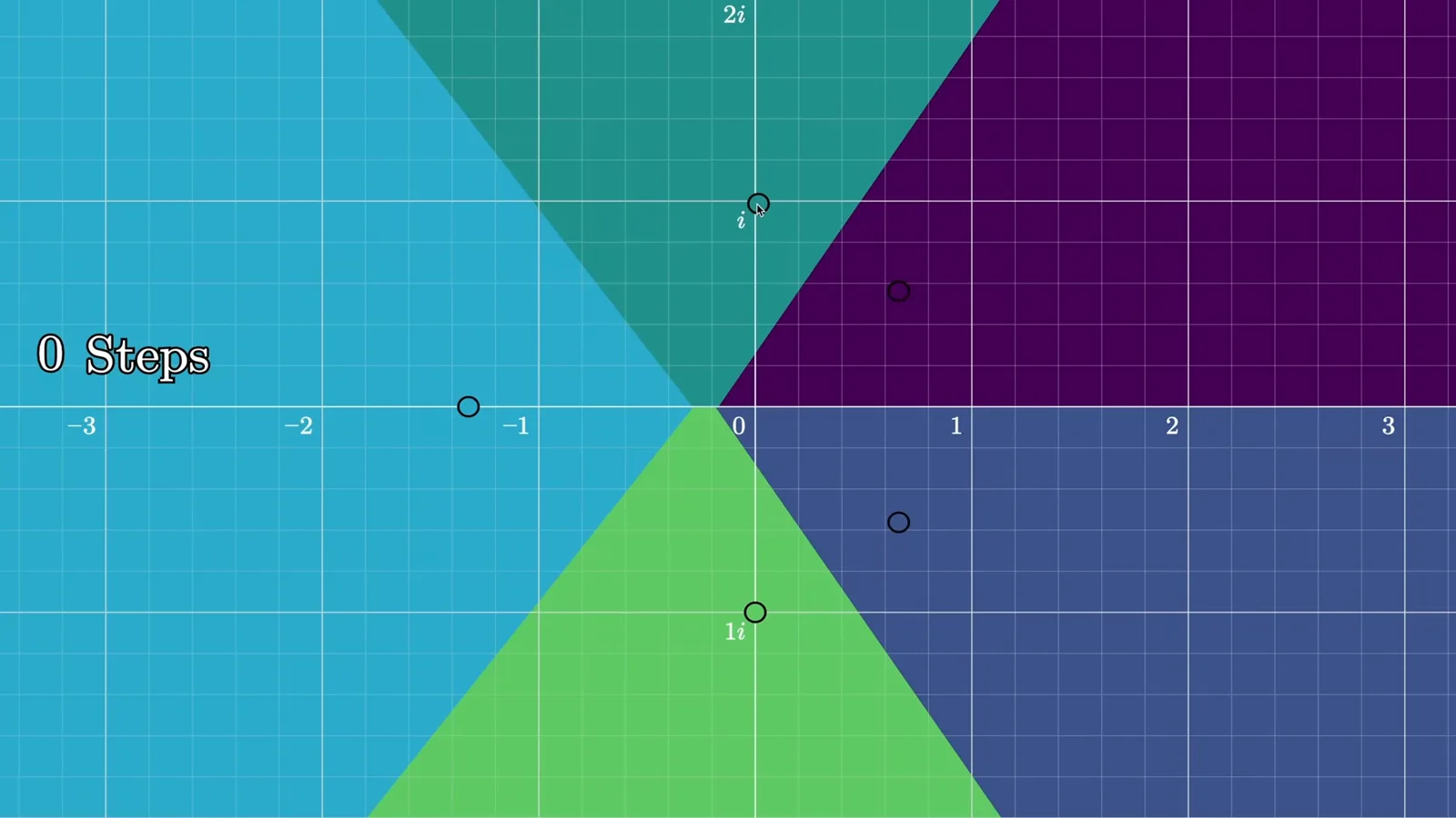
A useful comparison is to color each point by its nearest root without iterating at all. That gives a Voronoi diagram with straight boundaries. One Newton step changes the regions; more steps add detail. The mathematical object concerns the limiting behavior, not any single finite-step image.

The complexity is not a consequence of the impossibility of a general quintic formula. A cubic can also produce a fractal basin boundary. For a quadratic with two distinct roots, the pictured Newton basins instead divide along the line equidistant from them, with exceptional behavior on that boundary.

The speaker states a striking shared-boundary property for the root basins under discussion: the boundary of one root’s basin is also the boundary of every other root’s basin. A point is on a set’s boundary if every sufficiently small neighborhood contains points both inside and outside the set.

For the illustrated three-color case, any neighborhood of a shared boundary point contains starting points attracted to all three roots. This does not mean every point in the neighborhood converges to a root: boundary points and other exceptional orbits need separate treatment.

Imagine trying to draw three colored regions with the same boundary. If red and green touch along a smooth line, blue must somehow reach every part of that line too. Adding blue patches creates new boundaries that must also be approached by green, and repeating the correction leads to structure at ever smaller scales.

This gives intuition for why the illustrated boundary cannot contain an ordinary smooth segment separating only two basins. The speaker estimates the fractal dimension of the particular boundary shown at about 1.44; that number is for this example, not a universal dimension for every Newton fractal.

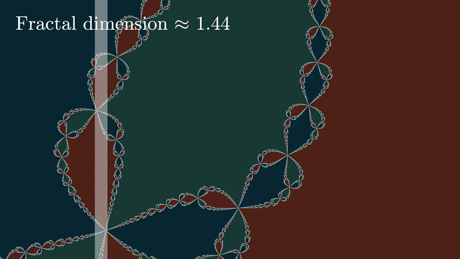
Translated back into root finding, near a shared boundary there are arbitrarily close initial guesses that lead to different roots, including every root basin. A cluster of guesses can stay together for several iterations and then spread widely before settling.

The two-root case can satisfy the shared-boundary condition with a smooth line because only two basins need meet. The condition alone does not force every two-color boundary to be smooth; it explains why the simple quadratic picture is compatible with the rule.

Why does the shared-boundary property hold? The speaker leaves the proof to a follow-up on holomorphic dynamics. The next video also explores whether Newton’s iteration can enter cycles and how that connects to the Mandelbrot set.

Newton never saw these modern images, just as many mathematical names later became attached to ideas their namesakes could not have anticipated. Even old methods can contain new questions waiting to be asked.